February 2, 2011I recently took the time out to rewrite the MVar documentation, which as it stands is fairly sparse (the introduction section rather tersely states “synchronising variables”; though to the credit of the original writers the inline documentation for the data type and its fundamental operations is fairly fleshed out.) I’ve reproduced my new introduction here.
While researching this documentation, I discovered something new about how MVars worked, which is encapsulated in this program. What does it do? :
import Control.Concurrent.MVar
import Control.Concurrent
main = do
    x <- newMVar 0
    forkIO $ do
        putMVar x 1
        putStrLn "child done"
    threadDelay 100
    readMVar x
    putStrLn "parent done"
An MVar t is mutable location that is either empty or contains a value of type t. It has two fundamental operations: putMVar which fills an MVar if it is empty and blocks otherwise, and takeMVar which empties an MVar if it is full and blocks otherwise. They can be used in multiple different ways:
- As synchronized mutable variables,
- As channels, with
takeMVar and putMVar as receive and send, and - As a binary semaphore
MVar (), with takeMVar and putMVar as wait and signal.
They were introduced in the paper “Concurrent Haskell” by Simon Peyton Jones, Andrew Gordon and Sigbjorn Finne, though some details of their implementation have since then changed (in particular, a put on a full MVar used to error, but now merely blocks.)
MVars offer more flexibility than IORefs, but less flexibility than STM. They are appropriate for building synchronization primitives and performing simple interthread communication; however they are very simple and susceptible to race conditions, deadlocks or uncaught exceptions. Do not use them if you need perform larger atomic operations such as reading from multiple variables: use ‘STM’ instead.
In particular, the “bigger” functions in this module (readMVar, swapMVar, withMVar, modifyMVar_ and modifyMVar) are simply compositions a takeMVar followed by a putMVar with exception safety. These only have atomicity guarantees if all other threads perform a takeMVar before a putMVar as well; otherwise, they may block.
The original paper specified that no thread can be blocked indefinitely on an MVar unless another thread holds that MVar indefinitely. This implementation upholds this fairness property by serving threads blocked on an MVar in a first-in-first-out fashion.
Like many other Haskell data structures, MVars are lazy. This means that if you place an expensive unevaluated thunk inside an MVar, it will be evaluated by the thread that consumes it, not the thread that produced it. Be sure to evaluate values to be placed in an MVar to the appropriate normal form, or utilize a strict MVar provided by the strict-concurrency package.
Consider the following concurrent data structure, a skip channel. This is a channel for an intermittent source of high bandwidth information (for example, mouse movement events.) Writing to the channel never blocks, and reading from the channel only returns the most recent value, or blocks if there are no new values. Multiple readers are supported with a dupSkipChan operation.
A skip channel is a pair of MVars: the second MVar is a semaphore for this particular reader: it is full if there is a value in the channel that this reader has not read yet, and empty otherwise.
import Control.Concurrent.MVar
import Control.Concurrent

data SkipChan a = SkipChan (MVar (a, [MVar ()])) (MVar ())

newSkipChan :: IO (SkipChan a)
newSkipChan = do
    sem <- newEmptyMVar
    main <- newMVar (undefined, [sem])
    return (SkipChan main sem)

putSkipChan :: SkipChan a -> a -> IO ()
putSkipChan (SkipChan main _) v = do
    (_, sems) <- takeMVar main
    putMVar main (v, [])
    mapM_ (\sem -> putMVar sem ()) sems

getSkipChan :: SkipChan a -> IO a
getSkipChan (SkipChan main sem) = do
    takeMVar sem
    (v, sems) <- takeMVar main
    putMVar main (v, sem:sems)
    return v

dupSkipChan :: SkipChan a -> IO (SkipChan a)
dupSkipChan (SkipChan main _) = do
    sem <- newEmptyMVar
    (v, sems) <- takeMVar main
    putMVar main (v, sem:sems)
    return (SkipChan main sem)
This example was adapted from the original Concurrent Haskell paper. For more examples of MVars being used to build higher-level synchronization primitives, see Control.Concurrent.Chan and Control.Concurrent.QSem.
December 31, 2010Here is to celebrate a year of blogging. Thank you all for reading. It was only a year ago that I first opened up shop under the wings of Iron Blogger. Iron Blogger has mostly disintegrated at this point, but I’m proud to say that this blog has not, publishing thrice a week, every week (excepting that one time I missed a post and made it up with a bonus post later that month), a bet that I made with myself and am happy to have won.
Where has this blog gone over the year? According to Google Analytics, here were the top ten most viewed posts:
- Graphs not grids: How caches are corrupting young algorithms designers and how to fix it
- You could have invented zippers
- Medieval medicine and computers
- Databases are categories
- Design Patterns in Haskell
- Static Analysis for everday (not-PhD) man
- MVC and purity
- Day in the life of a Galois intern
- Replacing small C programs with Haskell
- How to use Vim’s textwidth like a pro
There are probably a few obscure ones that are my personal favorites, but I’ve written so many at this point it’s a little hard to count: including this post, I will have published 159 posts, totaling somewhere around 120,000 words. (This figure includes markup, but for comparison, a book is about 80,000 words. Holy cow, I’ve written a book and a half worth of content. I don’t really feel like a better writer though—this may be because I’ve skimped on the “revising” bit of the process.)
This blog will go on a brief hiatus for the month of January. Not because I wouldn’t be able to produce posts over the holidays (given the chance, I probably would… in fact, this was a kind of hard decision to make) but because I should spend a month concentrating the bulk of my free time on stuff other than blogging. Have a happy New Years, and see you in February!
Postscript. Here is the SQL query I used to count:
select
  sum( length(replace(post_content, '  ', '')) - length(replace(post_content, ' ', ''))+1)
from wp_posts
where post_status = 'publish';
There’s probably a more accurate way of doing it, but I was too lazy to write out the script.
December 29, 2010“Roughing it,” so to speak.

With no reservations and no place to go, the hope was to crash somewhere in the Jungfrau region above the “fogline”

but these plans were thwarted by my discovery that Wengen had no hostels. Ah well.


Still pretty.
Of which I do not have a photo, one of the astonishing sights from Lauterbrunnen at night (I checked in and asked the owner, “Any open beds?” They replied, “One!” Only one possible response: “Excellent!”) is that the towns and trains interspersed on the mountains almost look like stars (the mountain hidden from view, due to their sparseness), clustered together in chromatic galaxies.
Non sequitur. A question for the readers: “What is a solution you have that is in search of a problem?”
December 27, 2010New to this series? Start at the beginning!
Recursion is perhaps one of the first concepts you learn about when you learn functional programming (or, indeed, computer science, one hopes.) The classic example introduced is factorial:
fact :: Int -> Int
fact 0 = 1 -- base case
fact n = n * fact (pred n) -- recursive case
Recursion on natural numbers is closely related to induction on natural numbers, as is explained here.
One thing that’s interesting about the data type Int in Haskell is that there are no infinities involved, so this definition works perfectly well in a strict language as well as a lazy language. (Remember that Int is a flat data type.) Consider, however, Omega, which we were playing around with in a previous post: in this case, we do have an infinity! Thus, we also need to show that factorial does something sensible when it is passed infinity: it outputs infinity. Fortunately, the definition of factorial is precisely the same for Omega (given the appropriate typeclasses.) But why does it work?
One operational answer is that any given execution of a program will only be able to deal with a finite quantity: we can’t ever actually “see” that a value of type Omega is infinity. Thus if we bound everything by some large number (say, the RAM of our computer), we can use the same reasoning techniques that applied to Int. However, I hope that you find something deeply unsatisfying about this answer: you want to think of an infinite data type as infinite, even if in reality you will never need the infinity. It’s the natural and fluid way to reason about it. As it turns out, there’s an induction principle to go along with this as well: transfinite induction.
recursion on natural numbers - induction
recursion on Omega - transfinite induction
Omega is perhaps not a very interesting data type that has infinite values, but there are plenty of examples of infinite data types in Haskell, infinite lists being one particular example. So in fact, we can generalize both the finite and infinite cases for arbitrary data structures as follows:
recursion on finite data structures - structural induction
recursion on infinite data structures - Scott induction
Scott induction is the punch line: with it, we have a versatile tool for reasoning about the correctness of recursive functions in a lazy language. However, its definition straight up may be a little hard to digest:
Let D be a cpo. A subset S of D is chain-closed if and only if for all chains in D, if each element of the chain is in S, then the least upper bound of the chain is in S as well. If D is a domain, a subset S is admissible if it is chain-closed and it contains bottom. Scott’s fixed point induction principle states that to prove that fix(f) is in S, we merely need to prove that for all d in D, if d is in S, then f(d) is in S.
When I first learned about Scott induction, I didn’t understand why all of the admissibility stuff was necessary: it was explained to me to be “precisely the stuff necessary to make the induction principle work.” I ended up coming around to this point of view in the end, but it’s a little hard to see in its full generality.
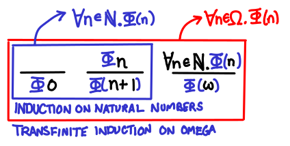
So, in this post, we’ll show how the jump from induction on natural numbers to transfinite induction corresponds to the jump from structural induction to Scott induction.
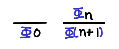
Induction on natural numbers. This is the induction you learn on grade school and is perhaps the simplest form of induction. As a refresher, it states that if some property holds for when n = 0, and if some property holds for n + 1 given that it holds for n, then the property holds for all natural numbers.
One way of thinking of the base case and the inductive step is to see them as inference rules that we need to show are true: if they are, we get another inference rule that lets us sidestep the infinite applications of the inductive step that would be necessary to satisfy ourselves that the property holds for all natural numbers. (Note that there is on problem if we only want to show that the property holds for an arbitrary natural number: that only requires a finite number of applications of the inductive step!)
Transfinite induction on Omega. Recall that Omega is the natural numbers plus the smallest infinite ordinal ω. Suppose that we wanted to prove that some property held for all natural numbers as well as infinity. If we just used induction on natural numbers, we’d notice that we’d be able to prove the property for some finite natural number, but not necessarily for infinity (for example, we might conclude that every natural number has another number greater than it, but there is no value in Omega greater than infinity).
This means we need one case: given that a property holds for all natural numbers, it holds for ω as well. Then we can apply induction on natural numbers and then infer that the property holds for infinity as well.
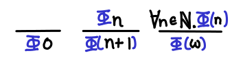
We notice that transfinite induction on Omega requires strictly more cases to be proven than induction on natural numbers, and as such is able to draw stronger conclusions.
Aside. In its full generality, we may have many infinite ordinals, and so the second case generalizes to successor ordinals (e.g. adding 1) and the third case generalizes to limit ordinal (that is, an ordinal that cannot be reached by repeatedly applying the successor function a finite number of times—e.g. infinity from zero). Does this sound familiar? I hope it does: this notion of a limit should remind you of the least upper bounds of chains (indeed, ω is the least upper bound of the only nontrivial chain in the domain Omega).
Let’s take a look at the definition of Scott induction again:
Let D be a cpo. A subset S of D is chain-closed if and only if for all chains in D, if each element of the chain is in S, then the least upper bound of the chain is in S as well. If D is a domain, a subset S is admissible if it is chain-closed and it contains bottom. Scott’s fixed point induction principle states that to prove that fix(f) is in S, we merely need to prove that for all d in D, if d is in S, then f(d) is in S.
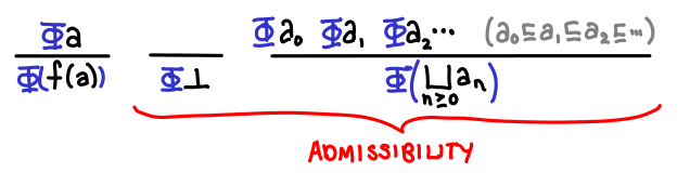
We can now pick out the parts of transfinite induction that correspond to statements in this definition. S corresponds to the set of values with the property we want to show, so S = {d | d in D and prop(d)} The base case is the inclusion of bottom in S. The successor case is “if d is in S, then f(d) is in S” (notice that f is our successor function now, not the addition of one). And the limit case corresponds to the chain-closure condition.
Here are all of the inference rules we need to show!
The domain D that we would use to prove that factorial is correct on Omega is the domain of functions Omega -> Omega, the successor function is (Omega -> Omega) -> (Omega -> Omega), and the subset S would correspond to the chain of increasingly defined versions of factorial. With all these ingredients in hand, we can see that fix(f) is indeed the factorial function we are looking for.
There are a number of interesting “quirks” about Scott induction. One is the fact that the property must hold for bottom, which is a partial correctness result (“such and such holds if the program terminates”) rather than a total correctness result (“the program terminates AND such and such holds”). The other is that the successor case is frequently not the most difficult part of a proof involving Scott induction: showing admissibility of your property is.
This concludes our series on denotational semantics. This is by no means complete: usually the next thing to look at is a simple functional programming language called PCF, and then relate the operational semantics and denotational semantics of this language. But even if you decide that you don’t want to hear any more about denotational semantics, I hope these glimpses into this fascinating world will help you reason about laziness in your Haskell programs.
Postscript. I originally wanted to relate all these forms of inductions to generalized induction as presented in TAPL: the inductive principle is that the least fixed point of a monotonic function F : P(U) -> P(U) (where P(U) denotes the powerset of the universe) is the intersection of all F-closed subsets of U. But this lead to the rather interesting situation where the greatest fixed points of functions needed to accept sets of values, and not just a single value. I wasn’t too sure what to make of this, so I left it out.
Unrelatedly, it would also be nice, for pedagogical purposes, to have a “paradox” that arises from incorrectly (but plausibly) applying Scott induction. Alas, such an example eluded me at the time of writing.
December 24, 2010How do you decide what to work on? I started thinking about this topic when I was wasting time on the Internet because I couldn’t think of anything to do that was productive. This seemed kind of strange: there were lots of things I needed to do: vacations to plan, projects to work on, support requests to answer, patches to merge in, theorems to prove, blog posts to write, papers to read, etc. So maybe the problem wasn’t that I didn’t have anything to do, it was just that I had too much stuff to do, and that I needed to pick something.
This choice is nontrivial. That evening, I didn’t feel like organizing my priorities either, so I just ended up just reading some comics, rationalizing it—erm, I mean filing it—under “Rest and Relaxation.” I could have chosen what to do based on some long term plan… yeah right, like I have a long time plan. It seems more practical to have chosen to do something enjoyable (which, when not involving reading comics, can occasionally involve productive work), or something that would give me a little high at the end, a kind of thrill from finishing—not necessarily fun when starting off, but fulfilling and satisfying by the end.
So what’s thrilling? In the famous book The Structure of Scientific Revolutions, Thomas Kuhn argued that what most scientists do is “normal science”, problem solving in the current field without any expectation of making revolutionary discoveries or changing the way we do science. This is a far cry from the idealistic vision ala “When I grow up, I want to be a scientist and discover a cure for cancer”—it would truly be thrilling to manage that. But if the life of an ordinary scientist is so mundane and so unlikely to result in a revolution, why do incredibly smart people dedicate their lives in the pursuit of scientific knowledge? What is thrilling about science?
Kuhn suggests that this may because humans love solving puzzles, and science is the ultimate puzzle solving activity: there is some hitherto unexplained phenomena, and a scientist attempts fit this phenomena into the existing theories and paradigms. And so while the average person may not find the in-depth analysis of a single section of DNA of a single obscure virus very interesting, for the scientist this generates endless puzzles for them to solve, each step of the way adding some knowledge, however small, to our civilization. And we humans find puzzles thrilling: they occupy us and give us that satisfaction when they are solved.
For a software engineer, the thrill may be in the creation of something that works and is useful to others (the rush of having users) or the thrill may be in having solved a particularly tricky problem (the rush that comes after you solve a tricky debugging session, or the rush when you do something very clever). The types of thrill you prefer dictate the kind of learning you are interested in. If you seek the thrill of creation, you will work on gaining the specialized knowledge of specific tools, libraries and applications that you will need in your craft. You will pursue knowledge outside of mere “programming”: aesthetics, design, psychology, marketing and more: the creation of a product is a truly interdisciplinary problem. If you seek the thrill of debugging (the hacker), you will seek specialized knowledge of a different kind, painstaking knowledge of the wire structure of protocols, source code, memory layout, etc. And if you seek the thrill of scientific problem solving, you will seek generalized, abstract knowledge, knowledge that suggests new ways of thinking about and doing things.
The steps towards each type of thrill are interrelated, but only to a certain degree. I remember a graduate student once telling me, “If you really want to make sure you understand something, you should go implement it. But sometimes this is counterproductive, because you spend so much time trying to make it work that you forget about the high level principles involved.” In this mindset, something becomes clear: not all knowledge is created equal. The first time I learn how to use a web framework, I acquire generalist knowledge—how a web framework might be put together, what functionality it is supposed to have and design idioms—as well as specialist knowledge—how this particular web framework works. But the next time I learn a different web framework, the generalist knowledge I gain is diminished. Repeat enough times, and all that’s left are implementation details: there is no element of surprise. (One caveat: at the limit, learning many, many web frameworks can give you some extra generalist knowledge simply by virtue of having seen so much. We might call this experience.)
For me, this presents an enormous conundrum. I want to create things! But creation requires contiguous chunks of time, which are rare and precious, and requires a constellation of generalist knowledge (the idea) and specialist knowledge (the details). So when I don’t have several weeks to devote to a single project (aka never), what should I do?
I’m not sure what I should do, but I have a vague sense for what my current rut is: alternate between working on projects that promise to give some generalist knowledge (whether it’s a short experiment for a blog post or hacking in the majestic mindbending landscape that is GHC) and slugging through my specialist maintenance workload. It… works, although it means I do a bit more writing and system administration than coding these days. C’est la vie.
December 21, 2010I will be in the following places at the following times:
- Paris up until evening of 12/22
- Berlin from 12/23 to 12/24
- Dresden on 12/24
- Munich from 12/25 to 12/26
- Zurich on 12/27
- Lucerne from 12/28 to 12/29
Plans over the New Year are still a little mushy, so I’ll post another update then. Let me know if you’d like to meet up!
Non sequitur. I went to the Mondrian exhibition at Centre Pompidou, and this particular gem, while not in the exhibition itself (it was in the female artists collection), I couldn’t resist snapping a photo of.

December 20, 2010What semantics has to say about specifications
Conventional wisdom is that premature generalization is bad (architecture astronauts) and vague specifications are appropriate for top-down engineering but not bottom-up. Can we say something a little more precise about this?
Semantics are formal specifications of programming languages. They are perhaps some of the most well-studied forms of specifications, because computer scientists love tinkering with the tools they use. They also love having lots of semantics to pick from: the more the merrier. We have small-step and big-step operational semantics; we have axiomatic semantics and denotational semantics; we have game semantics, algebraic semantics and concurrency semantics. Describing the programs we actually write is difficult business, and it helps to have as many different explanations as possible.
In my experience, it’s rather rare to see software have multiple specifications, each of them treated equally. Duplication makes it difficult to evolve the specification as more information becomes available and requirements change (as if it wasn’t hard enough already!) Two authoritative sources can conflict with each other. One version of the spec may dictate how precisely one part of the system is to be implemented, where the other leaves it open (up to some external behavior). What perhaps is more common is a single, authoritative specification, and then a constellation of informative references that you might actually refer to on a day-to-day basis.
Of course, this happens in the programming language semantics world all the time. On the subject of conflicts and differing specificity, here are two examples from denotational semantics (Scott semantics) and game semantics.
Too general? Here, the specification allows for some extra behavior (parallel or in PCF) that is impossible to implement in the obvious way (sequentially). This problem puzzled researchers for some time: if the specification is too relaxed, do you add the feature that the specification suggests (PCF+por), or do you attempt to modify the semantics so that this extra behavior is ruled out (logical relations)? Generality can be good, but it frequently comes at the cost of extra implementation complexity. In the case of parallel or, however, this implementation complexity is a threaded runtime system, which is useful for unrelated reasons.
Too vague? Here, the specification fails to capture a difference in behavior (seq and pseq are (Scott) semantically equivalent) that happens to be important operationally speaking (control of evaluation order). Game semantics neatly resolves this issue: we can distinguish between x `pseq` y and y `pseq` x because in the corresponding conversation, the expression asks for the value of x first in the former example, and the value of y first in the latter. However, vague specifications give more latitude to the compiler for optimizations.
Much like the mantra “the right language for the job”, I suspect there is a similar truth in “the right style of specification for the job.” But even further than that, I claim that looking at the same domain from different perspectives deepens your understanding of the domain itself. When using semantics, one includes some details and excludes others: as programmers we do this all the time—it’s critical for working on a system of any sort of complexity. When building semantics, the differences between our semantics give vital hints about the abstraction boundaries and potential inconsistencies in our original goals.
There is one notable downside to a lot of different paradigms for thinking about computation: you have to learn all of them! Axiomatic semantics recall the symbolic manipulation you might remember from High School maths: mechanical and not very interesting. Denotational semantics requires a bit of explaining before you can get the right intuition for it. Game semantics as “conversations” seems rather intuitive (to me) but there are a number of important details that are best resolved with some formality. Of course, we can always fall back to speaking operationally, but it is an approach that doesn’t scale for large systems (“read the source”).
December 17, 2010In which Edward travels France
Many, many years ago, I decided that I would study French rather than Spanish in High School. I wasn’t a particularly driven foreign language learner: sure I studied enough to get As (well, except for one quarter when I got a B+), but I could never convince myself to put enough importance on absorbing as much vocabulary and grammar as possible. Well, now I’m in France and this dusty, two-year old knowledge is finally being put to good use. And boy, am I wishing that I’d paid more attention in class.

Perhaps the first example of my fleeting French knowledge was when we reached the Marseille airport and I went up to the ticket counter and said, “Excusez-moi, je voudrais un… uhh…” the word for map having escaped my mind. I tried “carte” but that wasn’t quite correct. The agent helpfully asked me in English if I was looking for a map, to which I gratefully answered yes. Turns out the word is “plan.” I thanked the agent and consequently utterly failed to understand the taxi driver who took us to our first night’s accommodation in Plan-de-Cuques.
Still, my broken, incomplete knowledge of French was still better than none at all, and I soon recall enough about the imperatif and est-ce que to book a taxi, complain about coffee and tea we were served at Le Moulin Bleu (Tea bags? Seriously? Unfortunately, I was not fluent enough to get us a refund), and figure out what to do when we accidentally missed our bus stop (this involved me remembering what an eglise was). Though, I didn’t remember until Monday that Mercredi was Wednesday, not Monday.

Our itinerary involved staying in a few small French villages for the first few days, and then moving into the bigger cities (Lyon and Paris). Exploring small villages is a bit challenging, since the percentage of English speakers is much smaller and it’s easy to accidentally bus out to a town and find out that all of the stores are closed because it’s Monday and of course everything is closed on Monday! But there are also chances to be lucky: wandering out without any particular destination in mind, we managed to stumble upon a charming Christmas market and spontaneously climbed up a hill to a fantastic view of Marseilles.

Walking around in cold, subzero (Celsius) weather with your travel mates who have varying degrees of tolerance for physical exertion and the cold makes you empathize a bit with what your parents might have felt trucking you around as a kid during a vacation. After visiting the Basilica of Notre Dame in Lyon, I was somewhat at a loss for what to do next: the trip for shopping was a flop (none of us were particularly big shoppers), it was cold outside and the group didn’t have a particularly high tolerance for aimlessly wandering around a city. Spontaneity is difficult in a group. But it can happen, as it did when we trekked up to Tête d’Or and then cycled around with the Velo bike rent service (it’s “free” if you bike a half hour or less, but you have to buy a subscription, which for 1-day is one euro. Still quite a bargain.)

Teaching my travel mates phrases in French lead to perhaps one of the most serendipitous discoveries we made while at Lyon. We were up at Croix-de-Rousse at the indoors market, and it was 6:00; a plausible time for us British and American tourists to be thinking about dinner. I had just taught one of my travel mates how to ask someone if they spoke English (Vous parlez Anglais?) and she decided to find someone around who spoke English to ask for restaurant recommendations. The first few tries were a flop, but then we encountered an extremely friendly German visitor who was accompanied by a French native, and with it we got some restaurant recommendations, one of which was Balthaz’art, a pun on Balthasaur. After embarassingly banging on the door and being told they didn’t open until 7:30pm (right, the French eat dinner late), we decided to stick it out.

And boy was it worth it.


As for the title, noting the length of my blog posts, one of my MIT friends remarked, “Do you, like, do anything other than write blog posts these days?” To which I replied, “Tourist by day, Blogger by night”—since unlike many bloggers, I have not had the foresight to write up all of the posts for the next month in advance. Indeed, I need to go to sleep soon, since as of the time of writing (late Wednesday night), we train out to France tomorrow. Bonsoir, or perhaps for my temporally displaced East Coast readers, bonjour!
Photo credits. I nicked the lovely photo of Plan-de-Cuques from Gloria’s album. I’m still in the habit of being very minimalist when it comes to taking photos. (Stereotype of an Asian tourist! Well, I don’t do much better with my incredibly unchic ski jacket and snow pants.)
December 15, 2010New to this series? Start at the beginning!.
Today we’re going to take a closer look at a somewhat unusual data type, Omega. In the process, we’ll discuss how the lub library works and how you might go about using it. This is of practical interest to lazy programmers, because lub is a great way to modularize laziness, in Conal’s words.
Omega is a lot like the natural numbers, but instead of an explicit Z (zero) constructor, we use bottom instead. Unsurprisingly, this makes the theory easier, but the practice harder (but not too much harder, thanks to Conal’s lub library). We’ll show how to implement addition, multiplication and factorial on this data type, and also show how to prove that subtraction and equality (even to vertical booleans) are uncomputable.
This is a literate Haskell post. Since not all methods of the type classes we want to implement are computable, we turn off missing method warnings:
> {-# OPTIONS -fno-warn-missing-methods #-}
Some preliminaries:
> module Omega where
>
> import Data.Lub (HasLub(lub), flatLub)
> import Data.Glb (HasGlb(glb), flatGlb)
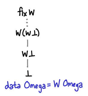
Here is, once again, the definition of Omega, as well as two distinguished elements of it, zero and omega (infinity.) Zero is bottom; we could have also written undefined or fix id. Omega is the least upper bound of Omega and is an infinite stack of Ws. :
> data Omega = W Omega deriving (Show)
>
> zero, w :: Omega
> zero = zero
> w    = W w -- the first ordinal, aka Infinity
Here are two alternate definitions of w:
w = fix W
w = lubs (iterate W zero)
The first alternate definition writes the recursion with an explicit fixpoint, as we’ve seen in the diagram. The second alternate definition directly calculates ω as the least upper bound of the chain [⊥, W ⊥, W (W ⊥) ...] = iterate W ⊥.
What does the lub operator in Data.Lub do? Up until now, we’ve only seen the lub operator used in the context of defining the least upper bound of a chain: can we usefully talk about the lub of two values? Yes: the least upper bound is simply the value that is “on top” of both the values.
If there is no value on top, the lub is undefined, and the lub operator may give bogus results.
If one value is strictly more defined than another, it may simply be the result of the lub.

An intuitive way of thinking of the lub operator is that it combines the information content of two expressions. So (1, ⊥) knows about the first element of the pair, and (⊥, 2) knows about the second element, so the lub combines this info to give (1, 2).
How might we calculate the least upper bound? One thing to realize is that in the case of Omega, the least upper bound is in fact the max of the two numbers, since this domain totally ordered. :
> instance Ord Omega where
>     max = lub
>     min = glb
Correspondingly, the minimum of two numbers is the greatest lower bound: a value that has less information content than both values.
If we think of a conversation that implements case lub x y of W a -> case a of W _ -> True, it might go something like this:
Me
Lub, please give me your value.
Lub
Just a moment. X and Y, please give me your values.
X
My value is W and another value.
Lub
Ok Edward, my value is W and another value.
Me
Thanks! Lub, what’s your next value?
Lub
Just a moment. X, please give me your next value.
Y
(A little while later.) My value is W and another value.
Lub
Ok. Y, please give me your next value.
Y
My next value is W and another value.
Lub
Ok Edward, my value is W and another value.
Me
Thanks!
X
My value is W and another value.
Lub
Ok.
Here is a timeline of this conversation:

There are a few interesting features of this conversation. The first is that lub itself is lazy: it will start returning answers without knowing what the full answer is. The second is that X and Y “race” to return a particular W, and lub will not act on the result that comes second. However, the ordering doesn’t matter, because the result will always be the same in the end (this will not be the case when the least upper bound is not defined!)
The unamb library that powers lub handles all of this messy, concurrency business for us, exposing it with the flatLub operator, which calculates the least upper bound for a flat data type. We need to give it a little help to calculate it for a non-flat data type (although one wonders if this could not be automatically derivable.) :
> instance Enum Omega where
>     succ = W
>     pred (W x) = x -- pred 0 = 0
>     toEnum n = iterate W zero !! n
>
> instance HasLub Omega where
>     lub x y = flatLub x y `seq` W (pred x `lub` pred y)
An equivalent, more verbose but more obviously correct definition is:
isZero (W _) = False -- returns ⊥ if zero (why can’t it return True?)
lub x y = (isZero x `lub` isZero y) `seq` W (pred x `lub` pred y)
It may also be useful to compare this definition to a normal max of natural numbers:
data Nat = Z | S Nat

predNat (S x) = x
predNat Z = Z

maxNat Z Z = Z
maxNat x y = S (maxNat (predNat x) (predNat y))
We can split the definition of lub into two sections: the zero-zero case, and the otherwise case. In maxNat, we pattern match against the two arguments and then return Z. We can’t directly pattern match against bottom, but if we promise to return bottom in the case that the pattern match succeeds (which is the case here), we can use seq to do the pattern match. We use flatLub and lub to do multiple pattern matches: if either value is not bottom, then the result of the lub is non-bottom, and we proceed to the right side of seq.
In the alternate definition, we flatten Omega into Bool, and then use a previously defined lub instance on it (we could have also used flatLub, since Bool is a flat domain.) Why are we allowed to use flatLub on Omega, which is not a flat domain? There are two reasons: the first is that seq only cares about whether or not the its first argument is bottom or not: it implicitly flattens all domains into “bottom or not bottom.” The second reason is that flatLub = unamb, and though unamb requires the values on both sides of it to be equal (so that it can make an unambiguous choice between either one), there is no way to witness the inequality of Omega: both equality and inequality are uncomputable for Omega. :
> instance Eq Omega where -- needed for Num
The glb instance rather easy, and we will not dwell on it further. The reader is encouraged to draw the conversation diagram for this instance. :
> instance HasGlb Omega where
>    glb (W x') (W y') = W (x' `glb` y')
This is a good point to stop and think about why addition, multiplication and factorial are computable on Omega, but subtraction and equality are not. If you take the game semantics route, you could probably convince yourself pretty well that there’s no plausible conversation that would get the job done for any of the latter cases. Let’s do something a bit more convincing: draw some pictures. We’ll uncurry the binary operators to help the diagrams.
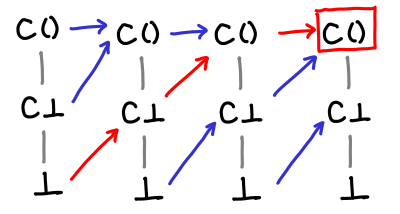
Here is a diagram for addition:
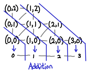
The pairs of Omega form a matrix (as usual, up and right are higher on the partial order), and the blue lines separate sets of inputs into their outputs. Multiplication is similar, albeit a little less pretty (there are a lot more slices).
We can see that this function is monotonic: once we follow the partial order into the next “step” across a blue line, we can never go back.
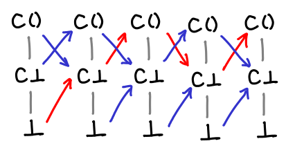
Consider subtraction now:
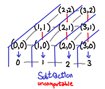
Here, the function is not monotonic: if I move right on the partial order and enter the next step, I can go “backwards” by moving up (the red lines.) Thus, it must not be computable.
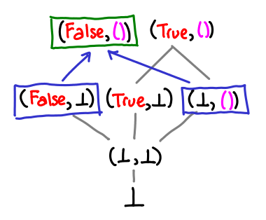
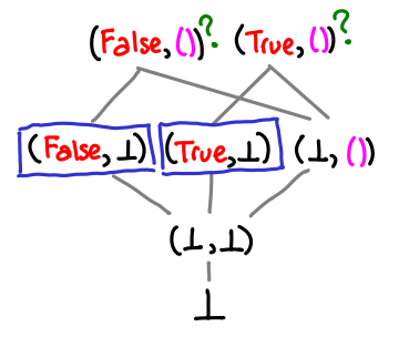
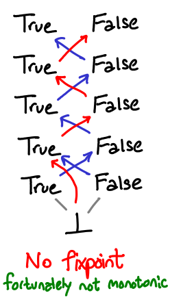
Here is the picture for equality. We immediately notice that mapping (⊥, ⊥) to True will mean that every value will have to map to True, so we can’t use normal booleans. However, we can’t use vertical booleans (with ⊥ for False and () for True) either:
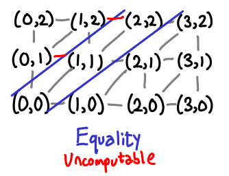
Once again, you can clearly see that this function is not monotonic.
It is now time to actually implement addition and multiplication:
> instance Num Omega where
>     x + y = y `lub` add x y
>         where add (W x') y = succ (x' + y)
>     (W x') * y = (x' * y) + y
>     fromInteger n = toEnum (fromIntegral n)
These functions look remarkably similar to addition and multiplication defined on Peano natural numbers:
natPlus Z y = y
natPlus (S x') y = S (natPlus x' y)

natMul Z y = Z
natMul (S x') y = natPlus y (natMul x' y)
There is the pattern matching on the first zero as before. But natPlus is a bit vexing: we pattern match against zero, but return y: our seq trick won’t work here! However, we can use the observation that add will be bottom if its first argument is bottom to see that if x is zero, then the return value will be y. What if x is not zero? We know that add x y must be greater than or equal to y, so that works as expected as well.
We don’t need this technique for multiplication because zero times any number is zero, and a pattern match will do that automatically for us.
And finally, the tour de force, factorial:
factorial n = W zero `lub` (n * factorial (pred n))
We use the same trick that was used for addition, noting that 0! = 1. For factorial 1, both sides of the lub are in fact equal, and for anything bigger, the right side dominates.
To sum up the rules for converting pattern matches against zero into lubs (assuming that the function is computable):
f ⊥ = ⊥
f (C x') = ...
becomes:
f (C x') = ...
(As you may have noticed, this is just the usual strict computation). The more interesting case:
g ⊥ = c
g (C x') = ...
becomes:
g x = c `lub` g' x
  where g' (C x') = ...
assuming that the original function g was computable (in particular, monotonic.) The case where x is ⊥ is trivial; and since ⊥ is at the bottom of the partial order, any possible value for g x where x is not bottom must be greater than or equal to bottom, fulfilling the second case.
A piece of frivolity. Quantum bogosort is a sorting algorithm that involves creating universes with all possible permutations of the list, and then destroying all universes for which the list is not sorted.
As it turns out, with lub it’s quite easy to accidentally implement the equivalent of quantum bogosort in your algorithm. I’ll use an early version of my addition algorithm to demonstrate:
x + y = add x y `lub` add y x
  where add (W x') y = succ (x' + y)
Alternatively, (+) = parCommute add where:
parCommute f x y = f x y `lub` f y x
This definition gets the right answer, but needs exponentially many threads to figure it out. Here is a diagram of what is going on:
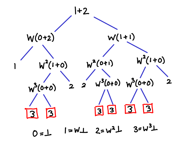
The trick is that we are repeatedly commuting the arguments to addition upon every recursion, and one of the nondeterministic paths leads to the result where both x and y are zero. Any other branch in the tree that terminates “early” will be less than the true result, and thus lub won’t pick it. Exploring all of these branches is, as you might guess, inefficient.
Next time, we will look at Scott induction as a method of reasoning about fixpoints like this one, relating it to induction on natural numbers and generalized induction. If I manage to understand coinduction by the next post, there might be a little on that too.
December 13, 2010Previously, we’ve drawn Hasse diagrams of all sorts of Haskell types, from data types to function types, and looked at the relationship between computability and monotonicity. In fact, all computable functions are monotonic, but not all monotonic functions are computable. Is there some description of functions that entails computability? Yes: Scott continuous functions. In this post, we look at the mathematical machinery necessary to define continuity. In particular, we will look at least upper bounds, chains, chain-complete partial orders (CPOs) and domains. We also look at fixpoints, which arise naturally from continuous functions.
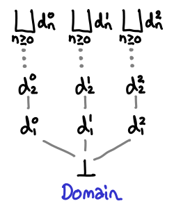
In our previous diagrams of types with infinitely many values, we let the values trail off into infinity with an ellipsis.
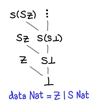
As several commentors have pointed out, this is not quite right: all Haskell data types also have a one or more top values, values that are not less than any other value. (Note that this is distinct from values that are greater than or equal to all other values: some values are incomparable, since these are partial orders we’re talking about.) In the case of Nat, there are a number of top values: Z, S Z, S (S Z), and so on are the most defined you can get. However, there is one more: fix S, aka infinity.
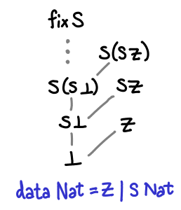
There are no bottoms lurking in this value, but it does seem a bit odd: if we peel off an S constructor (decrement the natural number), we get back fix S again: infinity minus one is apparently infinity.
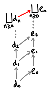
In fact, fix S is a least upper bound for the chain ⊥, S ⊥, S (S ⊥)… A chain is simply a sequence of values for which d_1 ≤ d_2 ≤ d_3 …; they are lines moving upwards on the diagrams we’ve drawn.
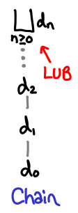
The least upper bound of a chain is just a value d which is bigger than all the members of the chain: it “sits at the top.” (For all n > 0, d_n ≤ d.) It is notated with a |_|, which is frequently called the “lub” operator. If the chain is strictly increasing, the least upper bound cannot be in the chain, because if it were, the next element in the chain would be greater than it.
A chain in a poset may not necessarily have a least upper bound. Consider the natural numbers with the usual partial ordering.
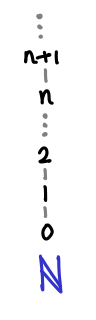
The chain 0 ≤ 1 ≤ 2 ≤ … does not have an upper bound, because the set of natural numbers doesn’t contain an infinity. We have to instead turn to Ω, which is the natural numbers and the smallest possible infinity, the ordinal ω.
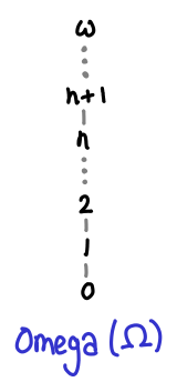
Here the chain has a least upper bound.
Despite not having a lub for 0 ≤ 1 ≤ 2 ≤ …, the natural numbers have many least upper bounds, since every element n forms the trivial chain n ≤ n ≤ n…
Here are pictorial representatios of some properties of lubs.
If one chain is always less than or equal to another chain, that chain’s lub is less than or equal to the other chain’s lub.
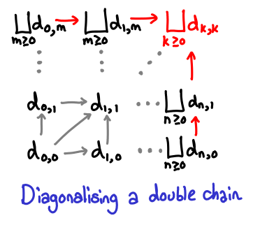
A double chain of lubs works the way you expect it to; furthermore, we can diagonalize this chain to get the upper bound in both directions.
So, if we think back to any of the diagrams we drew previously, anywhere there was a “…’, in fact we could have placed an upper bound on the top of, courtesy of Haskell’s laziness. Here is one chain in the list type that has a least upper bound:
As we saw earlier, this is not always true for all partial orders, so we have a special name for posets that always have least upper bounds: chain-complete posets, or CPOs.
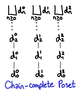
You may have also noticed that in every diagram, ⊥ was at the bottom. This too is not necessarily true of partial orders. We will call a CPO that has a bottom element a domain.
(The term domain is actually used quite loosely within the denotational semantics literature, many times having extra properties beyond the definition given here. I’m using this minimal definition from Marcelo Fiore’s denotational semantics lectures, and I believe that this is the Scott conception of a domain, although I haven’t verified this.)
So we’ve been in fact dealing with domains all this time, although we’ve been ignoring the least upper bounds. What we will find is that once we consider upper bounds we will find a stronger condition than monotonicity that entails computability.
Consider the following Haskell data type, which represents the vertical natural numbers Omega.
Here is a monotonic function that is not computable.
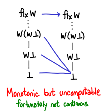
Why is it not computable? It requires us to treat arbitrarily large numbers and infinity different: there is a discontinuity between what happens on finite natural numbers and what happens at infinity. Computationally, there is no way for us to check in finite time that any given value we have is actually infinity: we can only continually keep peeling off Ws and hope we don’t reach bottom.
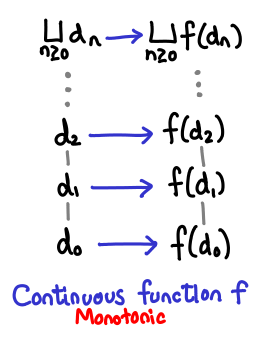
We can formalize this as follows: a function D -> D, where D is a domain, is continuous if it is monotonic and it preserves least upper bounds. This is not to say that the upper bounds all stay the same, but rather that if the upper bound of e_1 ≤ e_2 ≤ e_3 … is lub(e), then the upper bound of f(e_1) ≤ f(e_2) ≤ f(e_3) … is f(lub(e)). Symbolically:
$f(\bigsqcup_{n \ge 0} d_n) = \bigsqcup_{n \ge 0} f(d_n)$
Pictorially:
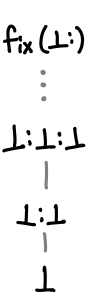
Now it’s time to look at fixpoints! We’ll jump straight to the punchline: Tarski’s fixpoint theorem states that the least fixed point of a continuous function is the least upper bound of the sequence ⊥ ≤ f(⊥) ≤ f(f(⊥)) …
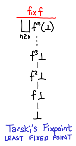
Because the function is continuous, it is compelled to preserve this least upper bound, automatically making it a fixed point. We can think of the sequence as giving us better and better approximations of the fixpoint. In fact, for finite domains, we can use this fact to mechanically calculate the precise fixpoint of a function.
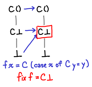
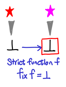
The first function we’ll look at doesn’t have a very interesting fixpoint.
If we pass bottom to it, we get bottom.
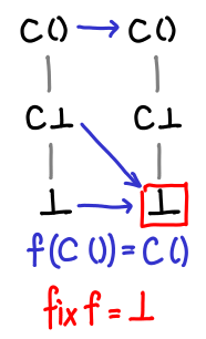
Here’s a slightly more interesting function.
It’s not obvious from the definition (although it’s more obvious looking at the Hasse diagrams) what the fixpoint of this function is. However, by repeatedly iterating f on ⊥, we can see what happens to our values:
Eventually we hit the fixpoint! And even more importantly, we’ve hit the least fixpoint: this particular function has another fixpoint, since f (C ()) = C ().
Here’s one more set for completeness.
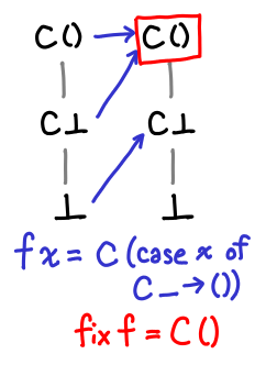
We can see from this diagrams a sort of vague sense why Tarski’s fixpoint theorem might work: we gradually move up and up the domain until we stop moving up, which is by definition the fixpoint, and since we start from the bottom, we end up with the least fixed point.
There are a few questions to answer. What if the function moved the value down? Then we might get stuck in an infinite loop.
We’re safe, however, because any such function would violate monotonicity: a loop on e₁ ≤ e₂ would result in f(e₁) ≥ f(e₂).
Our finite examples were also total orders: there was no branching of our diagrams. What if our function mapped a from one branch to another (a perfectly legal operation: think not)?
Fortunately, in order to get to such a cycle, we’d have to break monotonicity: a jump from one branch to another implies some degree of strictness. A special case of this is that the fixpoints of strict functions are bottom.
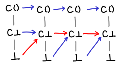
The tour de force example of fixpoints is the “Hello world” of recursive functions: factorial. Unlike our previous examples, the domain here is infinite, so fix needs to apply f “infinitely” many times to get the true factorial. Fortunately, any given call to calculuate the factorial n! will only need n applications. Recall that the fixpoint style definition of factorial is as follows:
factorial = fix (\f n -> if n == 0 then 1 else n * f (n - 1))
Here is how the domain of the factorial function grows with successive applications:
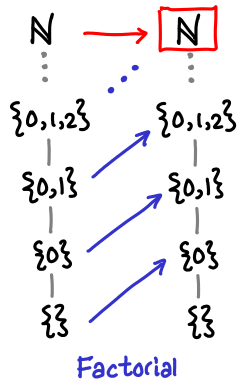
The reader is encouraged to verify this is the case. Next time, we’ll look at this example not on the flat domain of natural numbers, but the vertical domain of natural numbers, which will nicely tie to together a lot of the material we’ve covered so far.