February 23, 2011In his book Against Method, Paul Feyerabend writes the following provocative passage about ‘ad hoc approximations’, familiar to anyone whose taken a physics course and thought, “Now where did they get that approximation from…”
The perihelion of Mercury moves along at a rate of about 5600" per century. Of this value, 5026" are geometric, having to do with the movement of the reference system, while 531" are dynamical, due to the perturbations in the solar system. Of these perturbations all but the famous 43" are accounted for by classical mechanics. This is how the situation is usually explained.
The explanation shows that the premise from which we derive 43" is not the general theory of relativity plus suitable initial conditions. The premise contains classical physics in addition to whatever relativistic assumptions are being made. Furthermore, the relativistic calculation, the so-called ‘Schwarzschild solution’, does not deal with the planetary system as it exists in the real world (i.e. our own asymmetric galaxy); it deals with the entirely fictional case of a central symmetrical universe containing a singularity in the middle and nothing else. What are the reasons for employing such an odd conjunction of premises?
The reason, according to the customary reply, is that we are dealing with approximations. The formulae of classical physics do not appear because relativity is incomplete. Nor is the centrally symmetric case used because relativity does not offer anything better. Both schemata flow from the general theory under special circumstances realized in our planetary system provided we omit magnitudes too small to be considered. Hence, we are using the theory of relativity throughout, and we are using it in an adequate matter.
Note, how this idea of an approximation differs from the legitimate idea. Usually one has a theory, one is able to calculate the particular case one is interested in, one notes that this calculation leads to magnitudes below experimental precision, one omits such magnitudes, and one obtains a vastly simplified formalism. In the present case, making the required approximations would mean calculating the full n-body problem relativistically (including long-term resonances between different planetary orbits), omitting magnitudes smaller than the precision of observation reached, and showing that the theory thus curtailed coincides with classical celestial mechanics as corrected by Schwarzschild. This procedure has not been used by anyone simply because the relativistic n-body problem has as yet withstood solution. There are not even approximate solutions for important problems such as, for example, the problem of stability (one of the first great stumbling blocks for Newton’s theory). The classical part of the explanans [the premises of that explain our observations], therefore, does not occur just for convenience, it is absolutely necessary. And the approximations made are not a result of relativistic calculations, they are introduced in order to make relativity fit the case. One may properly call them ad hoc approximations.
Feyerabend is wonderfully iconoclastic, and I invite the reader to temporarily suspend their gut reaction to the passage. For those thinking, “Of course that’s what physicists do, otherwise we’d never get any work done,” consider the question, Why do we have any reason to believe that the approximations are justified, that they will not affect the observable results of our calculations, that they actually reflect reality? One could adopt the viewpoint that such doubts are unproductive and get in the way of doing science, which we know from prior experience to work. But I think this argument does have important implications for prescriptivists in all fields—those who would like to say how things ought to be done (goodness one sees a lot of that in the software field; even on this blog.) Because, just as the student complains, “There is no way I could have possibly thought up of that approximation” or the mathematician winces and thinks “There is no reason I should believe that approximation should work”, if these approximations do exist and the course of science is to discover them, well, how do you do that?
The ivory tower is not free of the blemishes of real life, it seems.
February 21, 2011When programmers automate something, we often want to go whole-hog and automate everything. But it’s good to remember there’s still a place for manual testing with machine assistance: instead of expending exponential effort to automate everything, automate the easy bits and hard-code answers to the hard research problems. When I was compiling the following graph of sources of test data, I noticed a striking polarization at the ends of “automated” and “non-automated.”

An ideal test framework would support combining all of these data sources and all of these testing mechanisms. Some novel approaches include:
- Randomly generated test-cases with manual verification. Obviously you won’t be able to hand verify thousands of test-cases, but a few concrete examples can do wonders for documentation purposes, and random generation prevents us from only picking “nice” inputs.
- Reference implementation as previous version of the code. To the limit, you automatically accept the output of an old implementation and save it to your test suite, and when a test starts failing you the framework asks you to check the output, and if it’s “better” than before you overwrite the old test data with the new. GHC’s test suite has something along these lines.
- You’ve written lots of algebraic laws, which you are using Quickcheck to verify. You should be able to swap out the random generator with a deterministic stream of data from a sampled data source. You’d probably want a mini-DSL for various source formats and transforming them into your target representation. This also works great when you’ve picked manual inputs, but exactly specifying the output result is a pain because it is large and complicated. This is data-driven testing.
- Non-fuzzing testing frameworks like Quickcheck and Smallcheck are reasonably good at dealing with runtime exceptions but not so much with more critical failures like segmentation faults. Drivers for these frameworks should take advantage of statelessness to notice when their runner has mysteriously died and let the user know the minimal invocation necessary to reproduce the crash—with this modification, these frameworks subsume fuzzers (which are currently built in an ad hoc fashion.)
It would be great if we didn’t have to commit to one testing methodology, and if we could reuse efforts on both sides of the fence for great victory.
February 20, 2011To: Oliver Charles
Subject: [Haskell-cafe] Please review my Xapian foreign function interface
Thanks Oliver!
I haven’t had time to look at your bindings very closely, but I do have a few initial things to think about:
- You’re writing your imports by hand. Several other projects used to do this, and it’s a pain in the neck when you have hundreds of functions that you need to bind and you don’t quite do it all properly, and then you segfault because there was an API mismatch. Consider using a tool like c2hs which rules out this possibility (and reduces the code you need to write!)
- I see a lot of unsafePerformIO and no consideration for interruptibility or thread safety. People who use Haskell tend to expect their code to be thread-safe and interruptible, so we have high standards ;-) But even C++ code that looks thread safe may be mutating shared memory under the hood, so check carefully.
I use Sup, so I deal with Xapian on a day-to-day basis. Bindings are good to see.
Cheers,
Edward
February 18, 2011Checked exceptions are a much vilified feature of Java, despite theoretical reasons why it should be a really good idea. The tension is between these two lines of reasoning:
Well-written programs handle all possible edge-cases, working around them when possible and gracefully dying if not. It’s hard to keep track of all possible exceptions, so we should have the compiler help us out by letting us know when there is an edge-case that we’ve forgotten to handle. Thus, checked exceptions offer a mechanism of ensuring we’ve handled all of the edge-cases.
and
Frequently checked exceptions are for error conditions that we cannot reasonably recover from close to the error site. Passing the checked exception through all of the intervening code requires each layer to know about all of its exceptions. The psychological design of checked exceptions encourages irresponsible swallowing of exceptions by developers. Checked exceptions don’t scale for large amounts of code.
In this post, I suggest another method for managing checked exceptions: prove that the code cannot throw such an exception.
“Prove that the code cannot throw an exception?” you might say. “Impossible! After all, most checked exceptions come from the outside world, and surely we can’t say anything about what will happen. A demon could just always pick the worst possible scenario and feed it into our code.”
My first answer to the skeptic would be that there do indeed exist examples of checked exceptions that happen completely deterministically, and could be shown to be guaranteed not to be thrown. For example, consider this code in the Java reflection API:
Object o, Field f; // defined elsewhere
f.setAccessible(true);
f.get(o);
The last invocation could throw a checked exception IllegalAccessException, but assuming that the setAccessible call did not fail (which it could, under a variety of conditions), this exception cannot happen! So, in fact, even if it did throw an IllegalAccessException, it has violated our programmer’s expectation of what the API should do and a nice fat runtime error will let us notice what’s going on. The call to setAccessible discharges the proof obligation for the IllegalAccessException case.
But this may just be an edge case in a world of overwhelmingly IO-based checked exceptions. So my second answer to the skeptic is that when we program code that interacts with the outside world, we often don’t assume that a demon is going to feed us the worst possible input data. (Maybe we should!) We have our own internal model of how the interactions might work, and if writing something that’s quick and dirty, it may be convenient to assume that the interaction will proceed in such and such a manner. So once we’ve written all the validation code to ensure that this is indeed the case (throwing a runtime exception akin to a failed assert if it’s not), we once again can assume static knowledge that can discharge our proof obligations. Yes, in a way it’s a cop out, because we haven’t proved anything, just told the compiler, “I know what I’m doing”, but the critical extra is that once we’ve established our assumptions, we can prove things with them, and only need to check at runtime what we assumed.
Of course, Java is not going to get dependent types any time soon, so this is all a rather theoretical discussion. But checked exceptions, like types, are a form of formal methods, and even if you don’t write your application in a dependently typed language, the field can still give useful insights about the underlying structure of your application.
The correspondence between checked exceptions and proofs came to me while listening to Conor McBride’s lecture on the Outrageous Arrows of Fortune. I hope to do a write up of this talk soon; it clarified some issues about session types that I had been thinking about.
I consulted the following articles when characterizing existing views of Java checked exceptions.
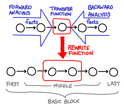
February 16, 2011Hoopl is a “higher order optimization library.” Why is it called “higher order?” Because all a user of Hoopl needs to do is write the various bits and pieces of an optimization, and Hoopl will glue it all together, the same way someone using a fold only needs to write the action of the function on one element, and the fold will glue it all together.
Unfortunately, if you’re not familiar with the structure of the problem that your higher order functions fit into, code written in this style can be a little incomprehensible. Fortunately, Hoopl’s two primary higher-order ingredients: transfer functions (which collect data about the program) and rewrite functions (which use the data to rewrite the program) are fairly easy to visualize.
February 14, 2011Guys, I have a secret to admit: I’m terrified of binomials. When I was in high school, I had a traumatic experience with Donald Knuth’s The Art of Computer Programming: yeah, that book that everyone recommends but no one has actually read. (That’s not actually true, but that subject is the topic for another blog post.) I wasn’t able to solve any recommended exercises in the mathematical first chapter nor was I well versed enough in computers to figure out what assembly languages were about. But probably the most traumatizing bit was Knuth’s extremely compact treatment of the mathematical identities in the first chapter we were expected memorize. As I would find out later in my mathematical career, it pays to convince yourself that a given statement is true before diving into the mess of algebraic manipulation in order to actually prove it.
One of my favorite ways of convincing myself is visualization. Heck, it’s even a useful way of memorizing identities, especially when the involve multiple parameters as binomial coefficients do. If I ever needed to calculate a binomial coefficient, I’d be more likely to bust out Pascal’s triangle than use the original equation.
Of course, at some point you have to write mathematical notation, and when you need to do that, reliance on the symmetric rendition of Pascal’s triangle (pictured on the right) can be harmful. Without peeking, the addition rule is obvious in Pascal’s triangle, but what’s the correct mathematical formulation?
[latex size=2]{n \choose k} = {n-1 \choose k} + {n-1 \choose k+1}[/latex]
[latex size=2]{n \choose k} = {n-1 \choose k-1} + {n-1 \choose k}[/latex]
I hate memorizing details like this, because I know I’ll get it wrong sooner or later if I’m not using the fact regularly (and while binomials are indubitably useful to the computer scientist, I can’t say I use them frequently.)
Pictures, however. I can remember pictures.
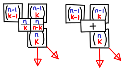
And if you visualize Pascal’s triangle as an actual table wih n on the y-axis and k on the x-axis, knowing where the spatial relationship of the boxes means you also know what the indexes are. It is a bit like visualizing dynamic programming. You can also more easily see the symmetry between a pair of equations like:
[latex size=2]{n \choose k} = {n \over k}{n-1 \choose k-1}[/latex]
[latex size=2]{n \choose k} = {n \over n-k}{n-1 \choose k}[/latex]
which are presented by the boxes on the left.
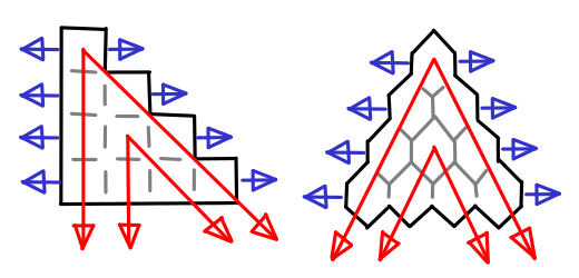
Of course, I’m not the first one to think of these visual aids. The “hockey stick identities” for summation down the diagonals of the traditional Pascal’s triangle are quite well known. I don’t think I’ve seen them pictured in tabular form, however. (I’ve also added row sums for completeness.)

Symmetry is nice, but unfortunately our notation is not symmetric, and so for me, remembering the hockey stick identities this ways saves me the trouble from then having to figure out what the indexes are. Though I must admit, I’m curious if my readership feels the same way.
February 11, 2011OpenIntents has a nifty application called SensorSimulator which allows you feed an Android application accelerometer, orientation and temperature sensor data. Unfortunately, it doesn’t work well on the newer Android 2.x series of devices. In particular:
- The mocked API presented to the user is different from the true API. This is due in part to the copies of the Sensor, SensorEvent and SensorEventHandler that the original code had in order to work around the fact that Android doesn’t have public constructors for these classes,
- Though the documentation claims “Whenever you are not connected to the simulator, you will get real device sensor data”, this is not actually the case: all of the code that interfaces with the real sensor system is commented out. So not only is are the APIs incompatible, you have to edit your code from one way to another when you want to vary testing. (The code also does a terrible job of handling the edge condition where you are not actually testing the application.)
Being rather displeased with this state of affairs, I decided to fix things up. With the power of Java reflection (cough cough) I switched the representation over to the true Android objects (effectively eliminating all overhead when the simulator is not connected.) Fortunately, Sensor and SensorEvent are small, data-oriented classes, so I don’t think I stepped on the internal representation too much, though the code will probably break horribly with future versions of the Android SDK. Perhaps I should suggest to upstream that they should make their constructors public.
You can grab the code here: SensorSimulator on Github. Let me know if you find bugs; I’ve only tested on Froyo (Android 2.2).
February 9, 2011To: John Wellesz
First off, I’d like to thank you for authoring the php.vim indentation plugin. Recent experiences with some other indentation plugins made me realize how annoying editing can be without a good indentation plugin, and php.vim mostly has served me well over the years.
However, I do have a suggestion for the default behavior of PHP_autoformatcomment. When this option is enabled (as it is by default), it sets the ‘w’ format option, which performs paragraphing based off of trailing newlines. Unfortunately, this option has a number of adverse effects that may not be obvious unless you are paying attention to trailing newlines:
When you are typing a comment, and you get an automatic linewrap, Vim will leave behind a single trailing whitespace to indicate “this is not the end of the paragraph!”
If you select a few adjacent comments, like such:
// Do this, but if you do that then
// be sure to frob the wibble
and then type ‘gq’, expecting it to be rewrapped, nothing will happen. This is because these lines lack trailing whitespace, so Vim thinks they are each a seperate sentence.
I also believe that ‘comments’ option should be unconditionally set by the indent plugin, as you load the ‘html’ plugin which clobbers any pre-existing value (specified, for example, by a .vim/indent/php.vim file).
Please let me know what you think of these changes. I also took a look at all the other indent scripts shipped with Vim by default and noted that none of them edit formatoptions.
February 7, 2011This picture snapped in Paris, two blocks from the apartment I holed up in. Some background.

February 4, 2011I spent some time fleshing out my count min sketch implementation for OCaml (to be the subject of another blog post), and along the way, I noticed a few more quirks about the OCaml language (from a Haskell viewpoint).
Unlike Haskell’s Int, which is 32-bit/64-bit, the built-in OCaml int type is only 31-bit/63-bit. Bit twiddlers beware! (There is a nativeint type which gives full machine precision, but it less efficient than the int type).
Semicolons have quite different precedence from the “programmable semicolon” of a Haskell do-block. In particular:
let rec repeat n thunk =
    if n == 0 then ()
    else thunk (); repeat (n-1) thunk
doesn’t do what you’d expect similarly phrased Haskell. (I hear I’m supposed to use begin and end.)
You can only get 30-bits of randomness from the Random module (an positive integer using Random.bits), even when you’re on a 64-bit platform, so you have to manually stitch multiple invocations to the generator together.
I don’t like a marching staircase of indentation, so I hang my “in”s after their statements—however, when they’re placed there, they’re easy to forget (since a let in a do-block does not require an in in Haskell).
Keyword arguments are quite useful, but they gunk up the type system a little and make it a little more difficult to interop keyword functions and non-keyword functions in a higher-order context. (This is especially evident when you’re using keyword arguments for documentation purposes, not because your function takes two ints and you really do need to disambiguate them.)
One observation about purity and randomness: I think one of the things people frequently find annoying in Haskell is the fact that randomness involves mutation of state, and thus be wrapped in a monad. This makes building probabilistic data structures a little clunkier, since you can no longer expose pure interfaces. OCaml is not pure, and as such you can query the random number generator whenever you want.
However, I think Haskell may get the last laugh in certain circumstances. In particular, if you are using a random number generator in order to generate random test cases for your code, you need to be able to reproduce a particular set of random tests. Usually, this is done by providing a seed which you can then feed back to the testing script, for deterministic behavior. But because OCaml’s random number generator manipulates global state, it’s very easy to accidentally break determinism by asking for a random number for something unrelated. You can work around it by manually bracketing the global state, but explicitly handling the randomness state means providing determinism is much more natural.