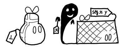
May 4, 2011When we teach beginners about Haskell, one of the things we handwave away is how the IO monad works. Yes, it’s a monad, and yes, it does IO, but it’s not something you can implement in Haskell itself, giving it a somewhat magical quality. In today’s post, I’d like to unravel the mystery of the IO monad by describing how GHC implements the IO monad internally in terms of primitive operations and the real world token. After reading this post, you should be able to understand the resolution of this ticket as well as the Core output of this Hello World! program:
main = do
    putStr "Hello "
    putStrLn "world!"
Nota bene: This is not a monad tutorial. This post assumes the reader knows what monads are! However, the first section reviews a critical concept of strictness as applied to monads, because it is critical to the correct functioning of the IO monad.
As a prelude to the IO monad, we will briefly review the State monad, which forms the operational basis for the IO monad (the IO monad is implemented as if it were a strict State monad with a special form of state, though there are some important differences—that’s the magic of it.) If you feel comfortable with the difference between the lazy and strict state monad, you can skip this section. Otherwise, read on. The data type constructor of the State monad is as follows:
newtype State s a = State { runState :: s -> (a, s) }
A running a computation in the state monad involves giving it some incoming state, and retrieving from it the resulting state and the actual value of the computation. The monadic structure involves threading the state through the various computations. For example, this snippet of code in the state monad:
do x <- doSomething
   y <- doSomethingElse
   return (x + y)
could be rewritten (with the newtype constructor removed) as:
\s ->
let (x, s')  = doSomething s
    (y, s'') = doSomethingElse s' in
(x + y, s'')
Now, a rather interesting experiment I would like to pose for the reader is this: suppose that doSomething and doSomethingElse were traced: that is, when evaluated, they outputted a trace message. That is:
doSomething s = trace "doSomething" $ ...
doSomethingElse s = trace "doSomethingElse" $ ...
Is there ever a situation in which the trace for doSomethingElse would fire before doSomething, in the case that we forced the result of the elements of this do block? In a strict language, the answer would obviously be no; you have to do each step of the stateful computation in order. But Haskell is lazy, and in another situation it’s conceivable that the result of doSomethingElse might be requested before doSomething is. Indeed, here is such an example of some code:
import Debug.Trace

f = \s ->
        let (x, s')  = doSomething s
            (y, s'') = doSomethingElse s'
        in (3, s'')

doSomething s = trace "doSomething" $ (0, s)
doSomethingElse s = trace "doSomethingElse" $ (3, s)

main = print (f 2)
What has happened is that we are lazy in the state value, so when we demanded the value of s'', we forced doSomethingElse and were presented with an indirection to s', which then caused us to force doSomething.
Suppose we actually did want doSomething to always execute before doSomethingElse. In this case, we can fix things up by making our state strict:
f = \s ->
        case doSomething s of
            (x, s') -> case doSomethingElse s' of
                          (y, s'') -> (3, s'')
This subtle transformation from let (which is lazy) to case (which is strict) lets us now preserve ordering. In fact, it will turn out, we won’t be given a choice in the matter: due to how primitives work out we have to do things this way. Keep your eye on the case: it will show up again when we start looking at Core.
Bonus. Interestingly enough, if you use irrefutable patterns, the case-code is equivalent to the original let-code:
f = \s ->
        case doSomething s of
            ~(x, s') -> case doSomethingElse s' of
                          ~(y, s'') -> (3, s'')
The next part of our story are the primitive types and functions provided by GHC. These are the mechanism by which GHC exports types and functionality that would not be normally implementable in Haskell: for example, unboxed types, adding together two 32-bit integers, or doing an IO action (mostly, writing bits to memory locations). They’re very GHC specific, and normal Haskell users never see them. In fact, they’re so special you need to enable a language extension to use them (the MagicHash)! The IO type is constructed with these primitives in GHC.Types:
newtype IO a = IO (State# RealWorld -> (# State# RealWorld, a #))
In order to understand the IO type, we will need to learn about a few of these primitives. But it should be very clear that this looks a lot like the state monad…
The first primitive is the unboxed tuple, seen in code as (# x, y #). Unboxed tuples are syntax for a “multiple return” calling convention; they’re not actually real tuples and can’t be put in variables as such. We’re going to use unboxed tuples in place of the tuples we saw in runState, because it would be pretty terrible if we had to do heap allocation every time we performed an IO action.
The next primitive is State# RealWorld, which will correspond to the s parameter of our state monad. Actually, it’s two primitives, the type constructor State#, and the magic type RealWorld (which doesn’t have a # suffix, fascinatingly enough.) The reason why this is divided into a type constructor and a type parameter is because the ST monad also reuses this framework—but that’s a matter for another blog post. You can treat State# RealWorld as a type that represents a very magical value: the value of the entire real world. When you ran a state monad, you could initialize the state with any value you cooked up, but only the main function receives a real world, and it then gets threaded along any IO code you may end up having executing.
One question you may ask is, “What about unsafePerformIO?” In particular, since it may show up in any pure computation, where the real world may not necessarily available, how can we fake up a copy of the real world to do the equivalent of a nested runState? In these cases, we have one final primitive, realWorld# :: State# RealWorld, which allows you to grab a reference to the real world wherever you may be. But since this is not hooked up to main, you get absolutely no ordering guarantees.
Let’s return to the Hello World program that I promised to explain:
main = do
    putStr "Hello "
    putStrLn "world!"
When we compile this, we get some core that looks like this (certain bits, most notably the casts (which, while a fascinating demonstration of how newtypes work, have no runtime effect), pruned for your viewing pleasure):
Main.main2 :: [GHC.Types.Char]
Main.main2 = GHC.Base.unpackCString# "world!"

Main.main3 :: [GHC.Types.Char]
Main.main3 = GHC.Base.unpackCString# "Hello "

Main.main1 :: GHC.Prim.State# GHC.Prim.RealWorld
              -> (# GHC.Prim.State# GHC.Prim.RealWorld, () #)
Main.main1 =
  \ (eta_ag6 :: GHC.Prim.State# GHC.Prim.RealWorld) ->
    case GHC.IO.Handle.Text.hPutStr1
           GHC.IO.Handle.FD.stdout Main.main3 eta_ag6
    of _ { (# new_s_alV, _ #) ->
    case GHC.IO.Handle.Text.hPutStr1
           GHC.IO.Handle.FD.stdout Main.main2 new_s_alV
    of _ { (# new_s1_alJ, _ #) ->
    GHC.IO.Handle.Text.hPutChar1
      GHC.IO.Handle.FD.stdout System.IO.hPrint2 new_s1_alJ
    }
    }

Main.main4 :: GHC.Prim.State# GHC.Prim.RealWorld
              -> (# GHC.Prim.State# GHC.Prim.RealWorld, () #)
Main.main4 =
  GHC.TopHandler.runMainIO1 @ () Main.main1

:Main.main :: GHC.Types.IO ()
:Main.main =
  Main.main4
The important bit is Main.main1. Reformatted and renamed, it looks just like our desugared state monad:
Main.main1 =
  \ (s :: State# RealWorld) ->
    case hPutStr1 stdout main3 s  of _ { (# s', _ #) ->
    case hPutStr1 stdout main2 s' of _ { (# s'', _ #) ->
    hPutChar1 stdout hPrint2 s''
    }}
The monads are all gone, and hPutStr1 stdout main3 s, while ostensibly always returning a value of type (# State# RealWorld, () #), has side-effects. The repeated case-expressions, however, ensure our optimizer doesn’t reorder the IO instructions (since that would have a very observable effect!)
For the curious, here are some other notable bits about the core output:
- Our
:main function (with a colon in front) doesn’t actually go straight to our code: it invokes a wrapper function GHC.TopHandler.runMainIO which does some initialization work like installing the top-level interrupt handler. unpackCString# has the type Addr# -> [Char], so what it does it transforms a null-terminated C string into a traditional Haskell string. This is because we store strings as null-terminated C strings whenever possible. If a null byte or other nasty binary is embedded, we would use unpackCStringUtf8# instead.putStr and putStrLn are nowhere in sight. This is because I compiled with -O, so these function calls got inlined.
To emphasize how important ordering is, consider what happens when you mix up seq, which is traditionally used with pure code and doesn’t give any order constraints, and IO, for which ordering is very important. That is, consider Bug 5129. Simon Peyton Jones gives a great explanation, so I’m just going to highlight how seductive (and wrong) code that isn’t ordered properly is. The code in question is x `seq` return (). What does this compile to? The following core:
case x of _ {
  __DEFAULT -> \s :: State# RealWorld -> (# s, () #)
}
Notice that the seq compiles into a case statement (since case statements in Core are strict), and also notice that there is no involvement with the s parameter in this statement. Thus, if this snippet is included in a larger fragment, these statements may get optimized around. And in fact, this is exactly what happens in some cases, as Simon describes. Moral of the story? Don’t write x `seq` return () (indeed, I think there are some instances of this idiom in some of the base libraries that need to get fixed.) The new world order is a new primop:
case seqS# x s of _ {
  s' -> (# s', () #)
}
Much better!
This also demonstrates why seq x y gives absolutely no guarantees about whether or not x or y will be evaluated first. The optimizer may notice that y always gives an exception, and since imprecise exceptions don’t care which exception is thrown, it may just throw out any reference to x. Egads!
- Most of the code that defines IO lives in the
GHC supermodule in base, though the actual IO type is in ghc-prim. GHC.Base and GHC.IO make for particularly good reading. - Primops are described on the GHC Trac.
- The ST monad is also implemented in essentially the exact same way: the unsafe coercion functions just do some type shuffling, and don’t actually change anything. You can read more about it in
GHC.ST.
May 2, 2011It is well known that unsafePerformIO is an evil tool by which impure effects can make their way into otherwise pristine Haskell code. But is the rest of Haskell really that pure? Here are a few questions to ask:
- What is the value of
maxBound :: Int? - What is the value of
\x y -> x / y == (3 / 7 :: Double) with 3 and 7 passed in as arguments? - What is the value of
os :: String from System.Info? - What is the value of
foldr (+) 0 [1..100] :: Int?
The answers to each of these questions are ill-defined—or you might say they’re well defined, but you need a little extra information to figure out what the actual result is.
- The Haskell 98 Report guarantees that the value of
Int is at least -2^29 to 2^29 - 1. But the precise value depends on what implementation of Haskell you’re using (does it need a bit for garbage collection purposes) and whether or not you’re on a 32-bit or 64-bit system. - Depending on whether or not the excess precision of your floating point registers is used to calculate the division, or if the IEEE standard is adhered to, this equality may or may not hold.
- Depending on what operating system the program is run on this value will change.
- Depending on the stack space allotted to this program at runtime, it may return a result or it may stack overflow.
In some respects, these constructs break referential transparency in an interesting way: while their values are guaranteed to be consistent during a single execution of the program, they may vary between different compilations and runtime executions of our program.
Is this kosher? And if it’s not, what are we supposed to say about the semantics of these Haskell programs?
The topic came up on #haskell, and I and a number of participants had a lively discussion about the topic. I’ll try to distill a few of the viewpoints here.
- The mathematical school says that all of this is very unsatisfactory, and that their programming languages should adhere to some precise semantics over all compilations and runtime executions. People ought to use arbitrary-size integers, and if they need modular arithmetic specify explicitly how big the modulus is (
Int32? Int64?) os is an abomination that should have been put in the IO sin bin. As tolkad puts it, “Without a standard you are lost, adrift in a sea of unspecified semantics. Hold fast to the rules of the specification lest you be consumed by ambiguity.” Limitations of the universe we live in are something of an embarrassment to the mathematician, but as long as the program crashes with a nice stack overflow they’re willing to live with a partial correctness result. An interesting subgroup is the distributed systems school which also care about the assumptions that are being made about the computing environment, but for a very practical reason. If multiple copies of your program are running on heterogeneous machines, you better not make any assumptions about pointer size on the wire. - The compile time school says that the mathematical approach is untenable for real world programming: one should program with compilation in mind. They’re willing to put up with a little bit of uncertainty in their source code programs, but all of the ambiguity should be cleared up once the program is compiled. If they’re feeling particularly cavalier, they’ll write their program with several meanings in mind, depending on the compile time options. They’re willing to put up with stack overflows, which are runtime determined, but are also a little uncomfortable with it. It is certainly better than the situation with
os, which could vary from runtime to runtime. The mathematicians make fun of them with examples like, “What about a dynamic linker or virtual machine, where some of the compilation is left off until runtime?” - The run time school says “Sod referential transparency across executions” and only care about internal consistency across a program run. Not only are they OK with stack overflows, they’re also OK with command line arguments setting global (pure!) variables, since those don’t change within the executions (they perhaps think
getArgs should have had the signature [String], not IO [String]), or variables that unsafely read in the contents of an external data file at program startup. They write things in docs like “This integer need not remain consistent from one execution of an application to another execution of the same application.” Everyone else sort of shudders, but it’s a sort of guilty pleasure that most people have indulged in at some point or another.
So, which school are you a member of?
Postscript. Since Rob Harper has recently posted another wonderfully iconoclastic blog post, and because his ending remarks are tangentially related to the topic of this post (purity), I thought I couldn’t help but sneak in a few remarks. Rob Harper states:
So why don’t we do this by default? Because it’s not such a great idea. Yes, I know it sounds wonderful at first, but then you realize that it’s pretty horrible. Once you’re in the IO monad, you’re stuck there forever, and are reduced to Algol-style imperative programming. You cannot easily convert between functional and monadic style without a radical restructuring of code. And you inevitably need unsafePerformIO to get anything serious done. In practical terms, you are deprived of the useful concept of a benign effect, and that just stinks!
I think Harper overstates the inability to write functional-style imperative programs in Haskell (conversions from functional to monadic style, while definitely annoying in practice, are relatively formulaic.) But these practical concerns do influence the day-to-day work of programmers, and as we’ve seen here, purity comes in all sorts of shades of gray. There is design space both upwards and downwards of Haskell’s current situation, but I think to say that purity should be thrown out entirely is missing the point.
April 29, 2011Today, we introduce the Grinch.

A formerly foul and unpleasant character, the Grinch has reformed his ways. He still has a penchant for stealing presents, but these days he does it ethically: he only takes a present if no one cares about it anymore. He is the garbage collector of the Haskell Heap, and he plays a very important role in keeping the Haskell Heap small (and thus our memory usage low)—especially since functional programs generate a lot of garbage. We’re not a particularly eco-friendly bunch.

The Grinch also collects garbage in traditional imperative languages, since the process is fundamentally the same. (We describe copying collection using Cheney’s algorithm here.) The Grinch first asks us what objects in the heap we care about (the roots). He moves these over to a new heap (evacuation), which will contain objects that will be saved. Then he goes over the objects in the new heap one by one, making sure they don’t point to other objects on the old heap. If they do, he moves those presents over too (scavenging). Eventually, he’s checked all of the presents in the new heap, which means everything left-over is garbage, and he drags it away.

But there are differences between the Haskell Heap and a traditional heap.
A traditional heap is one in which all of the presents have been opened: there will only be unwrapped boxes and gift-cards, so the Grinch only needs to check what gifts the gift-cards refer to in order to decide what else to scavenge.

However, the Haskell Heap has unopened presents, and the ghosts that haunt these presents are also pretty touchy when it comes to presents they know about. So the Grinch has to consult with them and scavenge any presents they point to.

How do presents become garbage? In both the Haskell Heap and a traditional heap, a present obviously becomes garbage if we tell the Grinch we don’t care about it anymore (the root set changes). Furthermore, if a gift-card is edited to point to a different present, the present it used to point to might also become unwanted (mutation). But what is distinctive about the Haskell Heap is this: after we open a present (evaluate a thunk), the ghost disappears into the ether, its job done. The Grinch may now be able to garbage collect the presents the ghost previously cared about.

Let’s review the life-cycle of a present on the Haskell Heap, in particular emphasizing the present’s relationship to other presents on the heap. (The phase names are actually used by GHC’s heap profiling.)

Suppose we want to minimize our memory usage by keeping the number of presents in our heap low. There are two ways to do this: we can reduce the number of presents we care about or we can reduce the number of presents we create. The former corresponds to making presents go dead, usually by opening a present and releasing any presents the now absent ghost cared about. The latter corresponds to avoiding function application, usually by not opening presents when unnecessary.
So, which one results in a smaller heap? It depends!

It is not true that only laziness causes space leaks on the heap. Excessive strictness can cause space leaks too. The key to fixing an identified space leak is figuring out which is the case. Nota bene: I’ve said a lot about space leaks, but I haven’t touched on a common space leak that plagues many people: space leaks on the stack. Stick around.
Last time: Functions produce the Haskell Heap
Next time: Bindings and CAFs on the Haskell Heap
Technical notes. The metaphor of the Grinch moving presents from one pile to another is only accurate if we assume copying garbage collections (GHC also has a compacting garbage collector, which operates differently), and some details (notably how the Grinch knows that a present has already been moved to the new heap, and how the Grinch keeps track of how far into the new heap he is) were skipped over. Additionally, the image of the Grinch “dragging off the garbage presents” is a little misleading: we just overwrite the old memory! Also, GHC doesn’t only have one heap: we have a generational garbage collector, which effectively means there are multiple heaps (and the Grinch visits the young heap more frequently than the old heaps.)
Presents and gift cards look exactly the same to a real garbage collector: a gift card is simply a pointer to a constructor info table and some pointer fields, whereas a present (thunk) is simply a pointer to the info table for the executable code and some fields for its closure variables. For Haskell, which treats data as code, they are one and the same. An implementation of anonymous functions in a language without them built-in might manually represent them as a data structure pointing to the static function code and extra space for its arguments. After all, evaluation of a lazy value is just a controlled form of mutation!

This work is licensed under a Creative Commons Attribution-ShareAlike 3.0 Unported License.
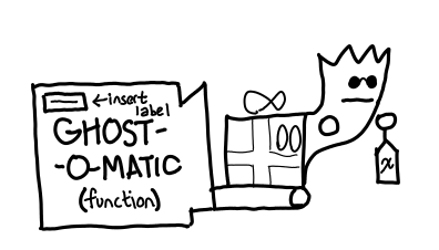
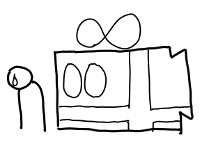
April 27, 2011We’ve talked about how we open (evaluate) presents (thunks) in the Haskell Heap: we use IO. But where do all of these presents come from? Today we introduce where all these presents come from, the Ghost-o-matic machine (a function in a Haskell program).

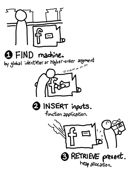
Using a function involves three steps.

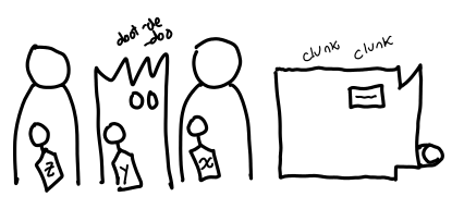
We can treat the machine as a black box that takes present labels and pops out presents, but you can imagine the inside as having an unlimited supply of identical ghosts and empty present boxes: when you run the machine, it puts a copy of the ghost in the box.

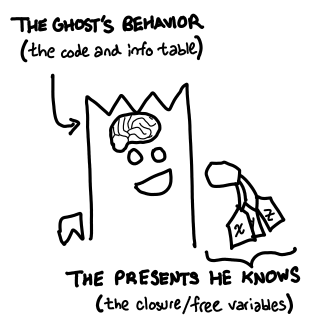
If the ghosts we put into the presents are identical, do they all behave the same way? Yes, but with one caveat: the actions of the ghost are determined by a script (the original source code), but inside the script there are holes that are filled in by the labels you inserted into the machine.

Since there’s not actually anything in the boxes, we can precisely characterize a present by the ghost that haunts it.

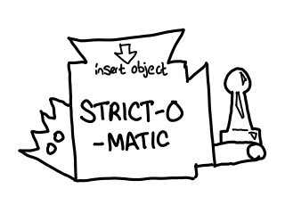
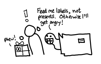
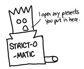
A frequent problem that people who use the Ghost-o-matic run into is that they expect it to work the same way as the Strict-o-matic (a function in a traditional, strictly evaluated language.) They don’t even take the same inputs: the Strict-o-matic takes unwrapped, unhaunted (unlifted) objects and gift cards, and outputs other unhaunted presents and gift cards.

But it’s really easy to forget, because the source-level syntax for strict function application and lazy function application are very similar.

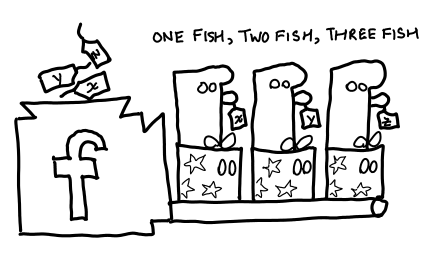
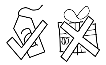
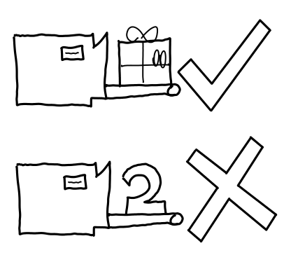
This is a point that must be thoroughly emphasized. In fact, in order to emphasize it, I’ve drawn two more pictures to reiterate what the permitted inputs and outputs for a Ghost-o-matic machine are.
Ghost-o-matics take labels of presents, not the actual presents themselves. This importantly means that the Ghost-o-matic doesn’t open any presents: after all, it only has labels, not the actual present. This stands in contrast to a Strict-o-matic machine which takes presents as inputs and opens them: one might call this machine the force function, of type Thunk a -> a. In Haskell, there is no such thing.

The Ghost-o-matic always creates a wrapped present. It will never produce an unwrapped present, even if there is no ghost haunting the present (the function was a constant).

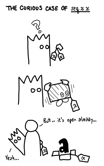
We state previously that there is no force function in Haskell. But the function seq seems to do something very like forcing a thunk. A present haunted by a seq ghost, when opened, will cause two other presents to be opened (even if the first one is unnecessary). It seems like the first argument is forced; and so seq x x might be some reasonable approximation of force in an imperative language. But what happens when we actually open up a present haunted by the seq ghost?

Although the ghost ends up opening the present rather than us, it’s too late for it to do any good: immediately after the ghost opens the present, we would have gone to open it (which it already is). The key observation is that the seq x x ghost only opens the present x when the present seq x x is opened, and immediately after seq x x is opened we have to go open x by means of an indirection. The strictness of the seq ghost is defeated by the fact that it’s put in a present, not to be opened until x is desired.
One interesting observation is that the Strict-o-matic machine does things when its run. It can open presents, fire missiles or do other side effects.

But the Ghost-o-matic machine doesn’t do any of that. It’s completely pure.
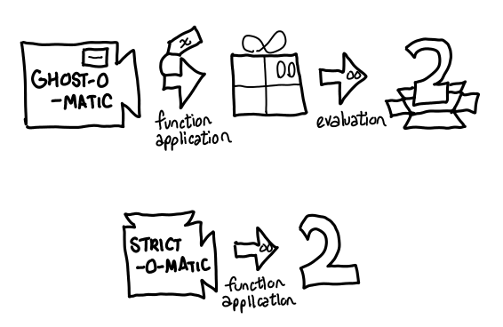
To prevent confusion, users of the Strict-o-matic and Ghost-o-matic machines may find it useful to compare the the present creation life-cycle for each of the machines.

The lazy Ghost-o-matic machine is split into two discrete phases: the function application, which doesn’t actually do anything, just creates the present, and the actual opening of the present. The Strict-o-matic does it all in one bang—although it could output a present (that’s what happens when you implement laziness inside a strict language). But in a strict language, you have to do it all yourself.
The Ghost-o-matic is approved for use by both humans and ghosts.

This does mean that opening a haunted present may produces more presents. For example, if the present produces a gift card for presents that don’t already live on the heap.

For a spine-strict data structure, it can produce a lot more presents.

Oh, and one more thing: the Ghost-o-matic makes a great gift for ghosts and family. They can be gift-wrapped in presents too. After all, everything in Haskell is a present.

Technical notes. With optimizations, a function may not necessarily allocate on the heap. The only way to be sure is to check out what optimized Core the program produces. It’s also not actually true that traditional, strict functions don’t exist in Haskell: unboxed primitives can be used to write traditional imperative code. It may look scary, but it’s not much different than writing your program in ML.
I’ve completely ignored partial application, which ought to be the topic of a later post, but I will note that, internally speaking, GHC does try its very best to pass all of the arguments a function wants at application time; if all the arguments are available, it won’t bother creating a partially application (PAP). But these can be thought of modified Ghost-o-matics, whose ghost already has some (but not all) of its arguments. Gifted ghost-o-matics (functions in the heap) can also be viewed this way: but rather than pre-emptively giving the ghost some arguments, the ghost is instead given its free variables (closure).
Last time: Implementing the Haskell Heap in Python, v1
Next time: How the Grinch stole the Haskell Heap

This work is licensed under a Creative Commons Attribution-ShareAlike 3.0 Unported License.
April 25, 2011Here is a simple implementation of all of the parts of the Haskell heap we have discussed up until now, ghosts and all.
heap = {} # global

# ---------------------------------------------------------------------#

class Present(object): # Thunk
    def __init__(self, ghost):
        self.ghost    = ghost # Ghost haunting the present
        self.opened   = False # Evaluated?
        self.contents = None
    def open(self):
        if not self.opened:
            # Hey ghost! Give me your present!
            self.contents = self.ghost.disturb()
            self.opened   = True
            self.ghost    = None
        return self.contents

class Ghost(object): # Code and closure
    def __init__(self, *args):
        self.tags = args # List of names of presents (closure)
    def disturb(self):
        raise NotImplemented

class Inside(object):
    pass
class GiftCard(Inside): # Constructor
    def __init__(self, name, *args):
        self.name  = name  # Name of gift card
        self.items = args # List of presents on heap you can redeem!
    def __str__(self):
        return " ".join([self.name] + map(str, self.items))
class Box(Inside): # Boxed, primitive data type
    def __init__(self, prim):
        self.prim = prim # Like an integer
    def __str__(self):
        return str(self.prim)

# ---------------------------------------------------------------------#

class IndirectionGhost(Ghost):
    def disturb(self):
        # Your present is in another castle!
        return heap[self.tags[0]].open()
class AddingGhost(Ghost):
    def disturb(self):
        # Gotta make your gift, be back in a jiffy!
        item_1 = heap[self.tags[0]].open()
        item_2 = heap[self.tags[1]].open()
        result = item_1.prim + item_2.prim
        return Box(result)
class UnsafePerformIOGhost(Ghost):
    def disturb(self):
        print "Fire ze missiles!"
        return heap[self.tags[0]].open()
class PSeqGhost(Ghost):
    def disturb(self):
        heap[self.tags[0]].open() # Result ignored!
        return heap[self.tags[1]].open()
class TraceGhost(Ghost):
    def disturb(self):
        print "Tracing %s" % self.tags[0]
        return heap[self.tags[0]].open()
class ExplodingGhost(Ghost):
    def disturb(self):
        print "Boom!"
        raise Exception

# ---------------------------------------------------------------------#

def evaluate(tag):
    print "> evaluate %s" % tag
    heap[tag].open()

def makeOpenPresent(x):
    present = Present(None)
    present.opened = True
    present.contents = x
    return present

# Let's put some presents in the heap (since we can't make presents
# of our own yet.)

heap['bottom']  = Present(ExplodingGhost())
heap['io']      = Present(UnsafePerformIOGhost('just_1'))
heap['just_1']  = makeOpenPresent(GiftCard('Just', 'bottom'))
heap['1']       = makeOpenPresent(Box(1))
heap['2']       = makeOpenPresent(Box(2))
heap['3']       = makeOpenPresent(Box(3))
heap['traced_1']= Present(TraceGhost('1'))
heap['traced_2']= Present(TraceGhost('2'))
heap['traced_x']= Present(TraceGhost('x'))
heap['x']       = Present(AddingGhost('traced_1', '3'))
heap['y']       = Present(PSeqGhost('traced_2', 'x'))
heap['z']       = Present(IndirectionGhost('traced_x'))

print """$ cat src.hs
import Debug.Trace
import System.IO.Unsafe
import Control.Parallel
import Control.Exception

bottom = error "Boom!"
io = unsafePerformIO (putStrLn "Fire ze missiles" >> return (Just 1))
traced_1 = trace "Tracing 1" 1
traced_2 = trace "Tracing 2" 2
traced_x = trace "Tracing x" x
x = traced_1 + 3
y = pseq traced_2 x
z = traced_x

main = do
    putStrLn "> evaluate 1"
    evaluate 1
    putStrLn "> evaluate z"
    evaluate z
    putStrLn "> evaluate z"
    evaluate z
    putStrLn "> evaluate y"
    evaluate y
    putStrLn "> evaluate io"
    evaluate io
    putStrLn "> evaluate io"
    evaluate io
    putStrLn "> evaluate bottom"
    evaluate bottom
$ runghc src.hs"""

# Evaluating an already opened present doesn't do anything
evaluate('1')

# Evaluating an indirection ghost forces us to evaluate another present
evaluate('z')

# Once a present is opened, it stays opened
evaluate('z')

# Evaluating a pseq ghost may mean extra presents get opened
evaluate('y')

# unsafePerformIO can do anything, but maybe only once..
evaluate('io')
evaluate('io')

# Exploding presents may live in the heap, but they're only dangerous
# if you evaluate them...
evaluate('bottom')
Technical notes. You can already see some resemblance of the ghosts’ Python implementations and the actual Core GHC might spit out. Here’s an sample for pseq:
pseq =
  \ (@ a) (@ b) (x :: a) (y :: b) ->
    case x of _ { __DEFAULT -> y }
The case operation on x corresponds to opening x, and once it’s open we do an indirection to y (return heap['y'].open()). Here’s another example for the non-polymorphic adding ghost:
add =
  \ (bx :: GHC.Types.Int) (by :: GHC.Types.Int) ->
    case bx of _ { GHC.Types.I# x ->
      case by of _ { GHC.Types.I# y ->
        GHC.Types.I# (GHC.Prim.+# x y)
      }
    }
In this case, Box plays the role of GHC.Types.I#. See if you can come up with some of the other correspondences (What is pattern matching on bx and by? What is GHC.Prim.+# ?)
I might do the next version in C just for kicks (and because then it would actually look something like what a real heap in a Haskell program looks like.)
Last time: IO evaluates the Haskell Heap
Next time: Functions produce the Haskell Heap

This work is licensed under a Creative Commons Attribution-ShareAlike 3.0 Unported License.
April 24, 2011In today’s post, we focus on you, the unwitting person rooting around the Haskell heap to open a present. After all, presents in the Haskell heap do not spontaneously unwrap themselves.

Someone has to open the first present.

If the Haskell heap doesn’t interact with the outside world, no presents need to be opened: thus IO functions are the ones that will open presents. What presents they will open is not necessarily obvious for many functions, so we’ll focus on one function that makes it particularly obvious: evaluate. Which tells you to…

…open a present.
If you get a primitive value, you’re done. But, of course, you might get a gift card (constructor):

Will you open the rest of the presents? Despite that deep, dissatisfaction inside you, the answer is no. evaluate only asks you to open one present. If it’s already opened, there’s nothing for you to do.

Advanced tip: If you want to evaluate more things, make a present containing a ghost who will open those things for you! A frequently used example of this when lazy IO is involved was evaluate (length xs), but don’t worry too much if you don’t understand that yet: I haven’t actually said how we make presents yet!
Even though we’re only opening one present, many things can happen, as described in the last post. It could execute some IO…

This is our direct window into evaluation as it evolves: when we run programs normally, we can’t see the presents being opened up; but if we ask the ghost to also shout out when it is disturbed, we get back this information. And in fact, this is precisely what Debug.Trace does!

There are other ways to see what evaluation is going on. A present could blow up: this is the exploding booby-trapped present, also known as “bottom”.

Perhaps the explosion was caused by an undefined or error "Foobar".

Boom.
We’ll end on a practical note. As we’ve mentioned, you can only be sure that a present has been opened if you’ve explicitly asked for it to be opened from IO. Otherwise, ghosts might play tricks on you. After all, you can’t actually see the Haskell heap, so there’s no way to directly tell if a present has been opened or not.

If you’re unsure when a thunk is being evaluated, add a trace statement to it. If ghosts are being lazy behind your back, the trace statement will never show up.

More frequently, however, the trace statement will show up; it’ll just be later than you expect (the ghosts may be lazy, but they’ll eventually get the job done.) So it’s useful to prematurely terminate your program or add extra print statements demarcating various stages of your program.
Last time: Evaluation on the Haskell Heap
Next time: Implementing the Haskell Heap in Python, v1
Technical notes. Contrary to what I’ve said earlier, there’s no theoretical reason why we couldn’t spontaneously evaluate thunks on the heap: this evaluation approach is called speculative evaluation. Somewhat confusingly, IO actions themselves can be thunks as well: this corresponds to passing around values of IO a without actually “running” them. But since I’m not here to talk about monads, I’ll simply ignore the existence of presents that contain IO actions—they work the same way, but you have to keep the levels of indirection straight. And finally, of course infinite loops also count as bottom, but the image of opening one present for the rest of eternity is not as flashy as an exploding present.

This work is licensed under a Creative Commons Attribution-ShareAlike 3.0 Unported License.
April 20, 2011
The Ghost of the Christmas Present
In today’s post, we’ll do a brief survey of the various things that can happen when you open haunted presents in the Haskell heap. Asides from constants and things that have already been evaluated, mostly everything on the Haskell heap is haunted. The real question is what the ghost haunting the present does.
In the simplest case, almost nothing!

Unlike gift-cards, you have to open the next present (Haskell doesn’t let you evaluate a thunk, and then decide not to follow the indirection…)

More commonly, the ghost was lazy and, when woken up, has to open other presents to figure out what was in your present in the first place!

Simple primitive operations need to open all of the presents involved.

But the ghost may also open another present for no particular reason…

or execute some IO…

Note that any presents he opens may trigger more ghosts:

Resulting in a veritable ghost jamboree, all to open one present!

The fact that opening a present (thunk) can cause such a cascading effect is precisely what makes the timing of lazy evaluation surprising to people who are used to all of the objects in their heap being unwrapped (evaluated) already. So the key to getting rid of this surprise is understanding when a ghost will decide it needs to unwrap a present (strictness analysis) and whether or not your presents are unwrapped already (amortized analysis).
Last time: The Haskell Heap
Next time: IO evaluates the Haskell Heap

This work is licensed under a Creative Commons Attribution-ShareAlike 3.0 Unported License.
April 18, 2011
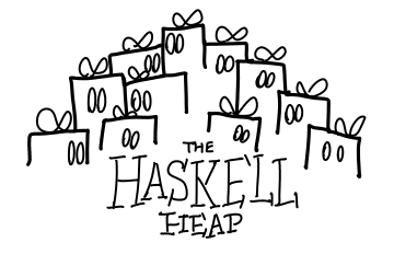
The Haskell heap is a rather strange place. It’s not like the heap of a traditional, strictly evaluated language…

…which contains a lot of junk! (Plain old data.)
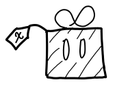
In the Haskell heap, every item is wrapped up nicely in a box: the Haskell heap is a heap of presents (thunks).

When you actually want what’s inside the present, you open it up (evaluate it).

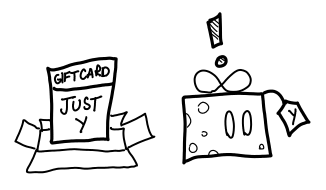
Presents tend to have names, and sometimes when you open a present, you get a gift card (data constructor). Gift cards have two traits: they have a name (the Just gift card or the Right gift card), and they tell you where the rest of your presents are. There might be more than one (the tuple gift card), if you’re a lucky duck!

But just as gift cards can lie around unused (that’s how the gift card companies make money!), you don’t have to redeem those presents.
Presents on the Haskell heap are rather mischievous. Some presents explode when you open them, others are haunted by ghosts that open other presents when disturbed.

Understanding what happens when you open a present is key to understanding the time and space behavior of Haskell programs.

In this series, Edward makes a foray into the webcomic world in order to illustrate the key operational concepts of evaluation in a lazily evaluated language. I hope you enjoy it!
Next time: Evaluation on the Haskell Heap
Technical notes. Technically speaking, this series should be “The GHC Heap.” However, I’ll try to avoid as many GHC-isms as possible, and simply offer a metaphor for operationally reasoning about any kind of lazy language. Originally, the series was titled “Bomberman Teaches Lazy Evaluation,” but while I’ve preserved the bomb metaphor for thunks that error or don’t terminate, I like the present metaphor better: it in particular captures several critical aspects of laziness: it captures the evaluated/non-evaluated distinction and the fact that once a present is opened, it’s opened for everyone. The use of the term “boxed” is a little suggestive: indeed, boxed or lifted values in GHC are precisely the ones that can be nonterminating, whereas unboxed values are more akin to what you’d see in C’s heap. However, languages like Java also use the term boxed to refer to primitive values that look like objects. For clarity’s sake, we won’t be using the term boxed from now on (indeed, we won’t mention unboxed types).

This work is licensed under a Creative Commons Attribution-ShareAlike 3.0 Unported License.
April 16, 2011What is the Mailbox? It’s a selection of interesting email conversations from my mailbox, which I can use in place of writing original content when I’m feeling lazy. I got the idea from Matt Might, who has a set of wonderful suggestions for low-cost academic blogging.
From: Brent Yorgey
I see you are a contributor to the sup mail client. At least I assume it is you, I doubt there are too many Edward Z. Yangs in the world. =) I’m thinking of switching from mutt. Do you still use sup? Any thoughts/encouragements/cautions to share?
To: Brent Yorgey
Yeah! I still use Sup, and I’ve blogged a little about it in the past, which is still essentially the setup I use. Hmm, some notes:
- I imagine that you want to switch away from Mutt because of some set of annoyances that has finally gotten unbearable. I will warn you that no mail client is perfect; many of my friends used to use Sup and gave up on it along the way. (I hear they use GMail now.) I’ve stuck it out, partially due to inertia, partially because someone else took ezyang@gmail.com, but also partially because I think it’s worth it :-)
- One of the things that has most dramatically changed the way I read email is the distinction between inbox and unread, and not-inbox and unread. In particular, while I have a fairly extensive set of filters that tag mail I get from mailing lists, when I read things on a day to day basis, I check my inbox for important stuff, and then I check my not-inbox “for fun”, mostly not reading most emails (but skimming the subject headers.) This means checking my mail in the morning is about a ten minute deal. This is the deal-maker for me.
- You will almost definitely want to setup OfflineIMAP, because downloading a 80 message thread from the Internet gets old very quickly. But Sup doesn’t propagate back changes to your mailbox this way (in particular, ‘read’ in Sup doesn’t mean ‘read’ in your INBOX) unless you use some experimental code on the maildir-sync branch. I’ve been using it for some time now quite well, but it does make getting other upstream changes a bit of an ordeal.
- Getting Sup setup will take some time; the initial import takes a long time and tweaking also takes a bit of time. Make sure you don’t have any deadlines coming soon. I’ve also found that it’s not really possible to use Sup without dipping your hand into some Ruby hacking (though maybe that’s just me :-); right now I have four hand-crafted patches on top of my source tree, and rebasing to master is not something done likely. I’ve actually gotten into a bit of trouble being so hack happy, but it’s also nice to be able to fix things when you need to (Sup not working is /very/ disruptive). Unfortunately, Ruby is not statically typed. :-)
Hope that helps. Do feel free to shout out if you need some help.
April 13, 2011It is often said that the factorial function is the “Hello World!” of the functional programming language world. Indeed, factorial is a singularly useful way of testing the pattern matching and recursive facilities of FP languages: we don’t bother with such “petty” concerns as input-output. In this blog post, we’re going to trace the compilation of factorial through the bowels of GHC. You’ll learn how to read Core, STG and Cmm, and hopefully get a taste of what is involved in the compilation of functional programs. Those who would like to play along with the GHC sources can check out the description of the compilation of one module on the GHC wiki. We won’t compile with optimizations to keep things simple; perhaps an optimized factorial will be the topic of another post!
The examples in this post were compiled with GHC 6.12.1 on a 32-bit Linux machine.
$ cat Factorial.hs
We start in the warm, comfortable land of Haskell:
module Factorial where

fact :: Int -> Int
fact 0 = 1
fact n = n * fact (n - 1)
We don’t bother checking if the input is negative to keep the code simple, and we’ve also specialized this function on Int, so that the resulting code will be a little clearer. But other then that, this is about as standard Factorial as it gets. Stick this in a file called Factorial.hs and you can play along.
$ ghc -c Factorial.hs -ddump-ds
Haskell is a big, complicated language with lots of features. This is important for making it pleasant to code in, but not so good for machine processing. So once we’ve got the majority of user visible error handling finished (typechecking and the like), we desugar Haskell into a small language called Core. At this point, the program is still functional, but it’s a bit wordier than what we originally wrote.
We first see the Core version of our factorial function:
Rec {
Factorial.fact :: GHC.Types.Int -> GHC.Types.Int
LclIdX
[]
Factorial.fact =
  \ (ds_dgr :: GHC.Types.Int) ->
    let {
      n_ade :: GHC.Types.Int
      LclId
      []
      n_ade = ds_dgr } in
    let {
      fail_dgt :: GHC.Prim.State# GHC.Prim.RealWorld -> GHC.Types.Int
      LclId
      []
      fail_dgt =
        \ (ds_dgu :: GHC.Prim.State# GHC.Prim.RealWorld) ->
          *_agj n_ade (Factorial.fact (-_agi n_ade (GHC.Types.I# 1))) } in
    case ds_dgr of wild_B1 { GHC.Types.I# ds_dgs ->
    letrec { } in
    case ds_dgs of ds_dgs {
      __DEFAULT -> fail_dgt GHC.Prim.realWorld#; 0 -> GHC.Types.I# 1
    }
    }
This may look a bit foreign, so here is the Core re-written in something that has more of a resemblance to Haskell. In particular I’ve elided the binder info (the type signature, LclId and [] that precede every binding), removed some type signatures and reindented:
Factorial.fact =
    \ds_dgr ->
        let n_ade = ds_dgr in
        let fail_dgt = \ds_dgu -> n_ade * Factorial.fact (n_ade - (GHC.Int.I# 1)) in
        case ds_dgr of wild_B1 { I# ds_dgs ->
            case ds_dgs of ds_dgs {
                __DEFAULT -> fail_dgt GHC.Prim.realWorld#
                0 -> GHC.Int.I# 1
            }
        }
It’s still a curious bit of code, so let’s step through it.
- There are no longer
fact n = ... style bindings: instead, everything is converted into a lambda. We introduce anonymous variables prefixed by ds_ for this purpose. - The first let-binding is to establish that our variable
n (with some extra stuff tacked on the end, in case we had defined another n that shadowed the original binding) is indeed the same as ds_dgr. It will get optimized away soon. - Our recursive call to
fact has been mysteriously placed in a lambda with the name fail_dgt. What is the meaning of this? It’s an artifact of the pattern matching we’re doing: if all of our other matches fail (we only have one, for the zero case), we call fail_dgt. The value it accepts is a faux-token GHC.Prim.realWorld#, which you can think of as unit. - We see that our pattern match has been desugared into a case-statement on the unboxed value of
ds_dgr, ds_dgs. We do one case switch to unbox it, and then another case switch to do the pattern match. There is one extra bit of syntax attached to the case statements, a variable to the right of the of keyword, which indicates the evaluated value (in this particular case, no one uses it.) - Finally, we see each of the branches of our recursion, and we see we have to manually construct a boxed integer
GHC.Int.I# 1 for literals.
And then we see a bunch of extra variables and functions, which represent functions and values we implicitly used from Prelude, such as multiplication, subtraction and equality:
$dNum_agq :: GHC.Num.Num GHC.Types.Int
LclId
[]
$dNum_agq = $dNum_agl
*_agj :: GHC.Types.Int -> GHC.Types.Int -> GHC.Types.Int
LclId
[]
*_agj = GHC.Num.* @ GHC.Types.Int $dNum_agq
-_agi :: GHC.Types.Int -> GHC.Types.Int -> GHC.Types.Int
LclId
[]
-_agi = GHC.Num.- @ GHC.Types.Int $dNum_agl
$dNum_agl :: GHC.Num.Num GHC.Types.Int
LclId
[]
$dNum_agl = GHC.Num.$fNumInt
$dEq_agk :: GHC.Classes.Eq GHC.Types.Int
LclId
[]
$dEq_agk = GHC.Num.$p1Num @ GHC.Types.Int $dNum_agl
==_adA :: GHC.Types.Int -> GHC.Types.Int -> GHC.Bool.Bool
LclId
[]
==_adA = GHC.Classes.== @ GHC.Types.Int $dEq_agk
fact_ado :: GHC.Types.Int -> GHC.Types.Int
LclId
[]
fact_ado = Factorial.fact
end Rec }
Since +, * and == are from type classes, we have to lookup the dictionary for each type dNum_agq and dEq_agk, and then use this to get our actual functions *_agj, -_agi and ==_adA, which are what our Core references, not the fully generic versions. If we hadn’t provided the Int -> Int type signature, this would have been a bit different.
ghc -c Factorial.hs -ddump-simpl
From here, we do a number of optimization passes on the core. Keen readers may have noticed that the unoptimized Core allocated an unnecessary thunk whenever n = 0, the fail_dgt. This inefficiency, among others, is optimized away:
Rec {
Factorial.fact :: GHC.Types.Int -> GHC.Types.Int
GblId
[Arity 1]
Factorial.fact =
  \ (ds_dgr :: GHC.Types.Int) ->
    case ds_dgr of wild_B1 { GHC.Types.I# ds1_dgs ->
    case ds1_dgs of _ {
      __DEFAULT ->
        GHC.Num.*
          @ GHC.Types.Int
          GHC.Num.$fNumInt
          wild_B1
          (Factorial.fact
             (GHC.Num.-
                @ GHC.Types.Int GHC.Num.$fNumInt wild_B1 (GHC.Types.I# 1)));
      0 -> GHC.Types.I# 1
    }
    }
end Rec }
Now, the very first thing we do upon entry is unbox the input ds_dgr and pattern match on it. All of the dictionary nonsense has been inlined into the __DEFAULT branch, so GHC.Num.* @ GHC.Types.Int GHC.Num.$fNumInt corresponds to multiplication for Int, and GHC.Num.- @ GHC.Types.Int GHC.Num.$fNumInt corresponds to subtraction for Int. Equality is nowhere to be found, because we could just directly pattern match against an unboxed Int.
There are a few things to be said about boxing and unboxing. One important thing to notice is that the case statement on ds_dgr forces this variable: it may have been a thunk, so some (potentially large) amount of code may run before we proceed any further. This is one of the reasons why getting backtraces in Haskell is so hard: we care about where the thunk for ds_dgr was allocated, not where it gets evaluated! But we don’t know that it’s going to error until we evaluate it.
Another important thing to notice is that although we unbox our integer, the result ds1_dgs is not used for anything other than pattern matching. Indeed, whenever we would have used n, we instead use wild_B1, which corresponds to the fully evaluated version of ds_dgr. This is because all of these functions expect boxed arguments, and since we already have a boxed version of the integer lying around, there’s no point in re-boxing the unboxed version.
ghc -c Factorial.hs -ddump-stg
Now we convert Core to the spineless, tagless, G-machine, the very last representation before we generate code that looks more like a traditional imperative program.
Factorial.fact =
    \r srt:(0,*bitmap*) [ds_sgx]
        case ds_sgx of wild_sgC {
          GHC.Types.I# ds1_sgA ->
              case ds1_sgA of ds2_sgG {
                __DEFAULT ->
                    let {
                      sat_sgJ =
                          \u srt:(0,*bitmap*) []
                              let {
                                sat_sgI =
                                    \u srt:(0,*bitmap*) []
                                        let { sat_sgH = NO_CCS GHC.Types.I#! [1];
                                        } in  GHC.Num.- GHC.Num.$fNumInt wild_sgC sat_sgH;
                              } in  Factorial.fact sat_sgI;
                    } in  GHC.Num.* GHC.Num.$fNumInt wild_sgC sat_sgJ;
                0 -> GHC.Types.I# [1];
              };
        };
SRT(Factorial.fact): [GHC.Num.$fNumInt, Factorial.fact]
Structurally, STG is very similar to Core, though there’s a lot of extra goop in preparation for the code generation phase:
- All of the variables have been renamed,
- All of the lambdas now have the form
\r srt:(0,*bitmap*) [ds_sgx]. The arguments are in the list at the rightmost side: if there are no arguments this is simply a thunk. The first character after the backslash indicates whether or not the closure is re-entrant (r), updatable (u) or single-entry (s, not used in this example). Updatable closures can be rewritten after evaluation with their results (so closures that take arguments can’t be updateable!) Afterwards, the static reference table is displayed, though there are no interesting static references in our program. NO_CCS is an annotation for profiling that indicates that no cost center stack is attached to this closure. Since we’re not compiling with profiling it’s not very interesting.- Constructor applications take their arguments in square brackets:
GHC.Types.I# [1]. This is not just a stylistic change: in STG, constructors are required to have all of their arguments (e.g. they are saturated). Otherwise, the constructor would be turned into a lambda.
There is also an interesting structural change, where all function applications now take only variables as arguments. In particular, we’ve created a new sat_sgJ thunk to pass to the recursive call of factorial. Because we have not compiled with optimizations, GHC has not noticed that the argument of fact will be immediately evaluated. This will make for some extremely circuitous intermediate code!
ghc -c Factorial.hs -ddump-cmm
Cmm (read “C minus minus”) is GHC’s high-level assembly language. It is similar in scope to LLVM, although it looks more like C than assembly. Here the output starts getting large, so we’ll treat it in chunks. The Cmm output contains a number of data sections, which mostly encode the extra annotated information from STG, and the entry points: sgI_entry, sgJ_entry, sgC_ret and Factorial_fact_entry. There are also two extra functions __stginit_Factorial_ and __stginit_Factorial which initialize the module, that we will not address.
Because we have been looking at the STG, we can construct a direct correspondence between these entry points and names from the STG. In brief:
sgI_entry corresponded to the thunk that subtracted 1 from wild_sgC. We’d expect it to setup the call to the function that subtracts Int.sgJ_entry corresponded to the thunk that called Factorial.fact on sat_sgI. We’d expect it to setup the call to Factorial.fact.sgC_ret is a little different, being tagged at the end with ret. This is a return point, which we will return to after we successfully evaluate ds_sgx (i.e. wild_sgC). We’d expect it to check if the result is 0, and either “return” a one (for some definition of “return”) or setup a call to the function that multiplies Int with sgJ_entry and its argument.
Time for some code! Here is sgI_entry:
sgI_entry()
        { has static closure: False update_frame: <none>
          type: 0
          desc: 0
          tag: 17
          ptrs: 1
          nptrs: 0
          srt: (Factorial_fact_srt,0,1)
        }
    ch0:
        if (Sp - 24 < SpLim) goto ch2;
        I32[Sp - 4] = R1; // (reordered for clarity)
        I32[Sp - 8] = stg_upd_frame_info;
        I32[Sp - 12] = stg_INTLIKE_closure+137;
        I32[Sp - 16] = I32[R1 + 8];
        I32[Sp - 20] = stg_ap_pp_info;
        I32[Sp - 24] = base_GHCziNum_zdfNumInt_closure;
        Sp = Sp - 24;
        jump base_GHCziNum_zm_info ();
    ch2: jump stg_gc_enter_1 ();
}
There’s a bit of metadata given at the top of the function, this is a description of the info table that will be stored next to the actual code for this function. You can look at CmmInfoTable in cmm/CmmDecl.hs if you’re interested in what the values mean; most notably the tag 17 corresponds to THUNK_1_0: this is a thunk that has in its environment (the free variables: in this case wild_sgC) a single pointer and no non-pointers.
Without attempting to understand the code, we can see a few interesting things: we are jumping to base_GHCziNum_zm_info, which is a Z-encoded name for base GHC.Num - info: hey, that’s our subtraction function! In that case, a reasonable guess is that the values we are writing to the stack are the arguments for this function. Let’s pull up the STG invocation again: GHC.Num.- GHC.Num.$fNumInt wild_sgC sat_sgH (recall sat_sgH was a constant 1).base_GHCziNum_zdfNumInt_closureis Z-encodedbase GHC.Num $fNumInt, so there is our dictionary function.stg_INTLIKE_closure+137is a rather curious constant, which happens to point to a statically allocated closure representing the number1. Which means at last we haveI32[R1 + 8], which must refer towild_sgC(in factR1is a pointer to this thunk’s closure on the stack.) You may ask, what dostg_ap_pp_infoandstg_upd_frame_infodo, and why isbase_GHCziNum_zdfNumInt_closureat the very bottom of the stack? The key is to realize that in fact, we’re placing three distinct entities on the stack: an argument forbase_GHCziNum_zm_info, astg_ap_pp_infoobject with a closure containingI32[R1 + 8]andstg_INTLIKE_closure+137, and astg_upd_frame_infoobject with a closure containingR1. We’ve delicately setup a Rube Goldberg machine, that when run, will do the following things: 1. Insidebase_GHCziNum_zm_info, consume the argumentbase_GHCziNum_zdfNumInt_closureand figure out what the right subtraction function for this dictionary is, put this function on the stack, and then jump to its return point, the next info table on the stack,stg_ap_pp_info. 2. Insidestg_ap_pp_info, consume the argument thatbase_GHCziNum_zm_infocreated, and apply it with the two argumentsI32[R1 + 8]andstg_INTLIKE_closure+137. (As you might imagine,stg_ap_pp_infois very simple.) 3. The subtraction function runs and does the actual subtraction. It then invokes the next info table on the stackstg_upd_frame_infowith this argument. 4. Because this is an updateable closure (remember theucharacter in STG?), willstg_upd_frame_infothe result of step 3 and use it to overwrite the closure pointed to byR1(the original closure of the thunk) with a new closure that simply contains the new value. It will then invoke the next info table on the stack, which was whatever was on the stack when we enteredsgI_Entry. Phew! And now there’s the minor question ofif (Sp - 24 < SpLim) goto ch2;which checks if we will overflow the stack and bugs out to the garbage collector if so.sgJ_entrydoes something very similar, but this time the continuation chain isFactorial_facttostg_upd_frame_infoto the great beyond. We also need to allocate a new closure on the heap (sgI_info), which will be passed in as an argument:: sgJ_entry() { has static closure: False update_frame: <none> type: 0 desc: 0 tag: 17 ptrs: 1 nptrs: 0 srt: (Factorial_fact_srt,0,3) } ch5: if (Sp - 12 < SpLim) goto ch7; Hp = Hp + 12; if (Hp > HpLim) goto ch7; I32[Sp - 8] = stg_upd_frame_info; I32[Sp - 4] = R1; I32[Hp - 8] = sgI_info; I32[Hp + 0] = I32[R1 + 8]; I32[Sp - 12] = Hp - 8; Sp = Sp - 12; jump Factorial_fact_info (); ch7: HpAlloc = 12; jump stg_gc_enter_1 (); } And finally,sgC_retactually does computation:: sgC_ret() { has static closure: False update_frame: <none> type: 0 desc: 0 tag: 34 stack: [] srt: (Factorial_fact_srt,0,3) } ch9: Hp = Hp + 12; if (Hp > HpLim) goto chb; _sgG::I32 = I32[R1 + 3]; if (_sgG::I32 != 0) goto chd; R1 = stg_INTLIKE_closure+137; Sp = Sp + 4; Hp = Hp - 12; jump (I32[Sp + 0]) (); chb: HpAlloc = 12; jump stg_gc_enter_1 (); chd: I32[Hp - 8] = sgJ_info; I32[Hp + 0] = R1; I32[Sp + 0] = Hp - 8; I32[Sp - 4] = R1; I32[Sp - 8] = stg_ap_pp_info; I32[Sp - 12] = base_GHCziNum_zdfNumInt_closure; Sp = Sp - 12; jump base_GHCziNum_zt_info (); } ...though not very much of it. We grab the result of the case split fromI32[R1 + 3](R1 is a tagged pointer, which is why the offset looks weird.) We then check if its zero, and if it is we shovestg_INTLIKE_closure+137(the literal 1) into our register and jump to our continuation; otherwise we setup our arguments on the stack to do a multiplicationbase_GHCziNum_zt_info. The same dictionary passing dance happens. And that’s it! While we’re here, here is a brief shout-out to “Optimised Cmm”, which is just Cmm but with some minor optimisations applied to it. If you’re *really* interested in the correspondence to the underlying assembly, this is good to look at. :: ghc -c Factorial.hs -ddump-opt-cmm Assembly ------------ :: ghc -c Factorial.hs -ddump-asm Finally, we get to assembly. It’s mostly the same as the Cmm, minus some optimizations, instruction selection and register allocation. In particular, all of the names from Cmm are preserved, which is useful if you’re debugging compiled Haskell code with GDB and don’t feel like wading through assembly: you can peek at the Cmm to get an idea for what the function is doing. Here is one excerpt, which displays some more salient aspects of Haskell on x86-32:: sgK_info: .Lch9: leal -24(%ebp),%eax cmpl 84(%ebx),%eax jb .Lchb movl $stg_upd_frame_info,-8(%ebp) movl %esi,-4(%ebp) movl $stg_INTLIKE_closure+137,-12(%ebp) movl 8(%esi),%eax movl %eax,-16(%ebp) movl $stg_ap_pp_info,-20(%ebp) movl $base_GHCziNum_zdfNumInt_closure,-24(%ebp) addl $-24,%ebp jmp base_GHCziNum_zm_info .Lchb: jmp *-8(%ebx) Some of the registers are pinned to registers we saw in Cmm. The first two lines are the stack check, and we can see that%ebpis always set to the value ofSp.84(%ebx)must be whereSpLim; indeed,%ebxstores a pointer to theBaseRegstructure, where we store various “register-like” data as the program executes (as well as the garbage collection function, see*-8(%ebx)). Afterwards, a lot of code moves values onto the stack, and we can see that%esicorresponds toR1. In fact, once you’ve allocated all of these registers, there aren’t very many general purpose registers to actually do computation in: just%eaxand%edx. Conclusion ------------- That’s it: factorial all the way down to the assembly level! You may be thinking several things: * *Holy crap! The next time I need to enter an obfuscated C contest, I’ll just have GHC generate my code for me.* GHC’s internal operational model is indeed very different from any imperative language you may have seen, but it is very regular, and once you get the hang of it, rather easy to understand. * *Holy crap! I can’t believe that Haskell performs at all!* Remember we didn’t compile with optimizations at all. The same module compiled with-O`` is considerably smarter.
Thanks for reading all the way! Stay tuned for the near future, where I illustrate action on the Haskell heap in comic book format.


