February 20, 2012Here is a full transcript to Github of Bret Victor’s “Inventing on Principle”. It was transcribed by me, An Yu and Tal Benisty.
Below is a copy of the transcript which I will endeavor to keep up to date with the Github copy. The original content was licensed under CC-BY.
[[0:07]] So, unlike the previous session, I don’t have any prizes to give out. I’m just going to tell you how to live your life.
[[0:14]] This talk is actually about a way of living your life that most people don’t talk about. As you approach your career, you’ll hear a lot about following your passion, or doing something you love. I’m going to talk about something kind of different. I’m going to talk about following a principle — finding a guiding principle for your work, something you believe is important and necessary and right, and using that to guide what you do.
[[0:46]] There are three parts to this talk. I’m first going to talk about the principle that guides a lot of my work, and try to give you a taste of what comes out of that. And I’m going to talk about some other people that have lived this way; what their principles are, what they believe in. But these are all just examples, to help you think about what you believe in, and how you want to live your life.
[[1:10]] So to begin with me: Ideas are very important to me. I think that bringing ideas into the world is one of the most important things that people do. And I think that great ideas, in the form of great art, stories, inventions, scientific theories, these things take on lives of their own, which give meaning to our lives as people. So, I think a lot about how people create ideas and how ideas grow. And in particular, what sorts of tools create a healthy environment for ideas to grow. Now, I’ve spent a lot of time over the years making creative tools, using creative tools, thinking about them a lot, and here’s something I’ve come to believe: Creators need an immediate connection to what they’re creating. That’s my principle. Creators need an immediate connection to what they create. And what I mean by that is when you’re making something, if you make a change, or you make a decision, you need to see the effect of that immediately. There can’t be a delay, and there can’t be anything hidden. Creators have to be able to see what they’re doing. Now I’m going to show a series of cases where I noticed that that principle was violated and I’ll show you what I did about that, and then I’m going to talk about the larger context in which I do this work.
[[2:32]] So, to begin with, let’s think about coding. Here’s how coding works: you type a bunch of code into a text editor, kind of imagining in your head what each line of code is going to do. And then you compile and run, and something comes out. So in this case, this is just JavaScript, drawing to a Canvas, and it draws this little scene with a tree. But if there’s anything wrong with the scene, or if I go and make changes, or if I have further ideas, I have to go back to the code, and I edit the code, compile and run, see what it looks like. Anything wrong, I go back to the code. Most of my time is spent working in the code, working in a text editor blindly, without an immediate connection to this thing, which is what I’m actually trying to make.
[[3:20]] So I feel that this goes against this principle that I have, that creators need an immediate connection to what they’re making, so I have tried to come up with a coding environment that would be more in line with this principle I have. So what I have here is I’ve got this picture on the side, and the code on the side, and this part draws the sky and this draws the mountains and this draws the tree, and when I make any change to the code, the picture changes immediately. So the code and the picture are always in sync; there is no compile and run. I just change things in the code and I see things change in the picture. And now that we have this immediate connection between the code and the picture, we can start thinking about ways of changing the code other than typing. So for example if this number here is the length of the branches. If I want to control that number, I just point my mouse to it, hold down the control key, and I can dial it up and down. So I can see what it looks like for big branches or small branches, and I can kind of converge on what feels right to me artistically. And this works great on any part of the code, I just point to it, and dial it up and down. Some of these numbers here, I know what they do but it’s kind of surprising to see them do it. [chuckles] And other ones are just completely surprising. [more chuckles]
[[4:48]] So down here, I’ve got this for loop where I’m counting to sixteen, I’m putting sixteen little pink blossoms on every branch. And I can turn it down for less blossoms or turn it up for more. But, look at what I’m doing here: I’m just kind of moving the number up and down around twenty or so: and it has this really interesting shimmering effect; it kind of looks as if the wind was blowing through the tree. And the first time I saw this I immediately started thinking about how I could use this effect for an animation. How would I ever have discovered that if I had to compile and run between every change? So much of art, so much of creation is discovery, and you can’t discover anything if you can’t see what you’re doing.
[[5:33]] So I’ve shown you adjusting the code, let’s add some code. I’d like to put a sun up here in the sky, so I’ll go to the end of the drawSky function, and I’ll want to fill a circle, so I start typing context.fillCircle, and as soon as I start typing, I get this autocomplete list of the different fill methods. So these are the things I can type there: fillCircle, fillRect, fillText. And as I move up and down this autocomplete list, I immediately see what each of them is doing. So, I don’t have to imagine what it would do from the method name. I don’t have to look at the documentation, I just see it, immediately.
[[6:12]] So I want a circle, and I’m going to adjust the x coordinate and the y coordinate, change the radius a bit. That looks about right. Probably it should be yellow, so I’m going to set the fill style, context.fillStyle, same autocomplete as before, choose fillStyle, gives me white by default, and I can change that color code the same way I change any number, I hit the control key, and I get a color palette. So I can choose a nice yellow for my sun. Although, the white was kind of interesting, I thought. I kind of didn’t expect that. But, with white, it now looks like the moon instead, right? Hey look, it’s night time! [chuckles] So having this immediate connection allows ideas to surface and develop in ways that would be impossible before.
[[7:17]] But there’s still a problem here, I think, which is I’ve got this picture, and I’ve got this code over here and I have to maintain the mapping between the two in my head. So I’ve got all these lines of code, and just looking at this line I don’t immediately know what it does. So here’s what I can do. I can hold down the option key, and my cursor changes to a magnifying glass, and now as I roll over each line of code, it’s highlighting in the picture what’s being drawn in that line. So, if I want to know what’s going on in this function, I just roll down the function and see what highlights. So here I’ve got two calls to drawMountain; I don’t know which is which; well, that’s that mountain, and that’s that mountain. And this has to work the other way too; if I see part of the picture, I have to know what code was responsible for drawing it. So I do the same thing; I hold down the option key, and now as I move over each pixel of the picture, you’ll see on the right it’s jumping to the line of code that drew that pixel. So that drew the sky, and that drew the tree, and that drew the blossom. So this is really important for maintaining that mapping, but it’s also really useful just for navigating around. So you know, I want to make the sun a little bit bigger; I jump there, and make it a little bigger. Or I want to bring up the tree a little bit; I jump there, and bring up the tree a little bit; I want to bring up the mountains a little bit, so I jump there, bring up the mountains a little bit; and I can make these changes as quickly as I think of them, and that is so important to the creative process. To be able to try ideas as you think of them. If there is any delay in that feedback loop, between thinking of something and seeing it, and building on it, then there is this whole world of ideas which will just never be. These are thoughts that we can’t think.
[[9:36]] Ideas are very important to me. And the thing about ideas is that ideas start small. Ideas start out tiny, weak and fragile. In order to develop and mature, ideas need an environment where the creator can nurture them. Kind of take care of them, feed them, and shape their growth. And to me, that’s what the principle of immediate connection is all about. And because ideas are so precious to me, when I see this principle violated, when I see ideas stillborn or stunted because their creator couldn’t see what they were doing, I feel that’s wrong. And not wrong in the sense of violating some UI guideline or going against some best practice, but wrong in a deeper sense then that. And I’ll come back to this, but I want to show you another example of following this principle.
[[10:26]] So in this code here, there is no state, there is no persistent state, there is no time, there is no interactivity. And I was thinking about how we would handle those aspects of coding in a way that’s in line with these principles I have: creators need immediate connection. So what I have here is a little platform game. Here is my little guy, he can run around, he can jump, he can die [chuckles]. And the code for him is over here. So this code makes him run around, this makes him jump, this makes him collide with things… and down here, I’ve got some code for this little turtle. And the turtle is not doing much right now because I haven’t finished writing his code, so, I’m just going to do that right now. Say on each tick his x position plus equals his direction times the time interval, one sixtieth of a second times some speed, which, um, I dunno? Could be fast, could be slow, if it’s negative, he walks backwards. [chuckles] And these are all ideas I can use for other enemies but I think turtles are supposed to be slow, so let’s set that speed for our turtle. And up here, I’ve got some code that says, when my guy collides with the turtle, he gets some Y velocity, so he bounces into the air, and the turtle gets stomped. So that looks like that. And the turtle gets up after a bit.
[[12:01]] The problem is, I don’t want the player to be able to get up here yet. I want the player to bounce off the turtle, and go through this little passageway down here. And he’ll have to go around and solve puzzles and whatnot, and then come back and get the star. So, the turtle is too bouncy right now. Now of course I can just turn that down on the code, and now I can try it but now it’s not bouncy enough. So while it’s nice that I can adjust the code while it’s running, without having to stop and recompile and find my place again, I can’t immediately see what I need to see, which is whether or not he can make that jump.
[[12:43]] So here’s what I’m going to do. I’m going to bounce off the turtle, and pause the game. So I pause the game, and now there’s this slider up here, which lets me rewind through time. And now, I can rewind to back before I made the jump, and change the code, make it less bouncy, and now when I move it forward, it’s going to simulate it, using the same input controls, the same keyboard commands recorded as before, but with the new code. [applause]
[[13:20]] This is not good enough. [laughter] I need to be able to see the changes immediately. I need to be able to see immediately whether or not my bounciness is correct. None of this stuff. And if you have a process in time, and you want to see changes immediately, you have to map time to space. So here’s what I’m going to do. I’m going to bounce off my turtle, pause the game, and now hit this button here, which shows my guy’s trail. So now I can see where he’s been. And when I rewind, this trail in front of him is where he is going to be. This is his future. And when I change the code, I change his future. [gasps] So I can find exactly the value I need, so when I hit play, he slips right in there. [applause]
[[14:26]] So, creators need to be able to see what they’re doing. If you’re designing something embedded in time you need to be able to control time. You need to be able to see across time, otherwise you’re designing blind.
[[14:40]] As I was playing with this, I noticed it’s fun to play with gravity. So I can make gravity a little negative and he starts to float up in the air. [laughter] And I can kind of play with that and try to get him to stay there. And you could probably make an entire game around just the mechanic here, it’s gravity manipulation. In fact, I bet I could fiddle with any part of this code and come up with an idea for a game. Even if I just comment out the first statement in the code, now my guy can’t move left - he can only move right. Which sounds kinda silly, but Terry Cavanagh actually made a beautiful game around that concept called “Don’t Look Back”. Terry Cavanagh, he made another really wonderful game which you might have seen, called “VVVVVV”, spelled as the letter v six times. And, the way that game works, is that you can’t jump. Instead, you can only flip upside down, and you fall up instead of falling down. So it kinda works like this. You can walk on the ceiling or you can walk around on the ground. And so you have these levels which kinda look like this, and you kinda walk around… You have to learn how to navigate a terrain like this. And so if you had like a, something like that, you wouldn’t be able to jump over it. You’d have to flip over and flip over; he got an amazing amount of gameplay out of this concept.
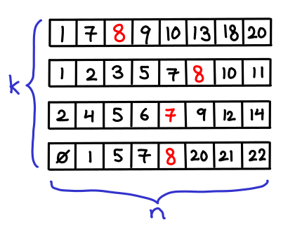
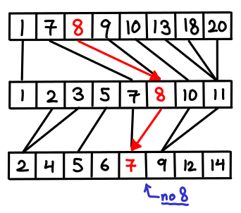
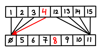
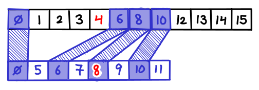
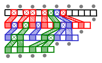
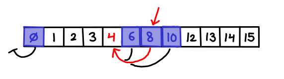
[[16:07]] So again, being able to try ideas as you think of them. [pause] This example, and the last one with the tree, these are both very visual programs; we’re able to see our changes just by seeing how the picture changes. So I was thinking about, how we could do more abstract coding that’s more in line with this principle. How can we write a generic algorithm in such a way that we can see what we’re doing. So as an example, let’s take a look at binary search. Super quick refresher on how binary search works: you have an array of values that are in order, and you have a key, which is the value you’re trying to locate within the array. And you keep track of two variables, which are the lower and upper bounds of where you think that value could possibly be; right now, it could be anywhere. And you look right in the middle of that range - if what you find is too small, then the key has to be after that. Look in the middle of the range, if what you find is too big, the key has to be before that. And you kinda keep subdividing your range until you narrow in on the value you’re looking for. And in code, binary search looks like this. And from my perspective, you can’t see anything here. You can’t see anything. I see the word ‘array’, but I don’t actually see an array. And so in order to write code like this, you have to imagine an array in your head, and you essentially have to play computer. You have to simulate in your head what each line of code would do on a computer. And to a large extent, the people that we consider to be skilled software engineers are just those people that are really good at playing computer. But if we’re writing our code on a computer… why are we simulating what a computer would do in our head? Why doesn’t the computer just do it… and show us?
[[18:06]] So. Let’s write binary search. Function “binary search” takes a key and an array. And then over here on this side, it’s saying “Ok, it takes a key and an array, such as what? Give me an example; I need something to work with here.” So, for instance, my array might be ‘a’, ‘b’, ‘c’, ’d’, ’e’, ‘f’. And let’s say for instance we’re looking for the ’d’. So now let’s start coding. The lower bound starts out as zero. Over here it says ’low equals zero’, nothing amazing there. Upper bound starts out at the end of the array, so high equals array length minus one. And over here, it says ‘high equals five’. So I have my abstract formula in the code. Over here, it’s giving me the concrete value corresponding to these example arguments. So I don’t have to maintain this picture in my head; it’s just showing it to me.
[[19:09]] So now I need the index in the middle of the array, so I’m going to take the average of those two. Mid equals low plus high over two, and… well, that’s obviously not right. Two point five is not a valid array index. So I guess I need to round this off. So I’m going to add the floor function and it rounded it down to two. And I caught that bug literally the second I typed it, instead of writing the entire function in twenty unit tests. So now I get the value out of the array… and then I need to subdivide my range, which, so there’s an if statement which I’ll just paste in here. So in this case, the value I found is less than the key, so it’s taking this first branch of the if statement. This is adjusting the lower bound. Of course if the key was smaller, then it would take this branch of the if statement and adjust the upper bound. Or, if the key was ‘c’, then we would’ve just happened to find it on the first shot, and we’d return the index.
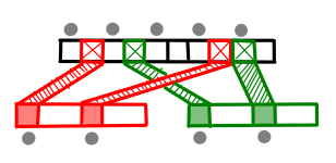
[[20:14]] So this is the first iteration of this algorithm. And now what we need to do, is loop. We’ve subdivided the array, we need to keep subdividing until we narrow in on what we’re looking for. So, we need to loop; I will just loop. While 1, do all this. And now what we have are three columns corresponding to three iterations of this loop. So this first column here is exactly what you saw before. Low and high span the entire array, we found a ‘c’, it was too low, so we adjusted our lower bound, and loop up to here. Second iteration, bounds are tighter; we found an ’e’. Adjust the upper bound. Third iteration, loop up to here; low and high are the same. We’ve narrowed it down to a single candidate - it’s indeed the key we’re looking for, and we returned this index. So there’s nothing hidden here; you see exactly what the algorithm is doing at every point. And I can go up to here and try different keys, so I can see how the algorithm behaves for these different input arguments.
[[21:20]] And by looking across this data, I can develop an intuition for how this algorithm works. So I’m trying different keys here, and say I try looking for a ‘g’. And this looks a little different. It’s not actually returning. And the reason for this is, I’m looking for a key which is not actually in the array. And the only way of breaking out of this loop, is by finding the key. So it’s kinda stuck here looping forever. So we can take a look at this and see what went wrong, where’s the algorithm going off the rails. These first few iterations look fine, but this iteration looks weird, because low is greater than high. Our range is completely collapsed. So if we get to this point, then we know the key can’t be found. So I see this faulty condition, and I say, “Oh, that’s not right; low has to be less than or equal to high.” Okay, well, I’ll just put that over as the condition of my while statement. Low, less than equal to high, and then that would break out of the loop, and I would return some signal to say that it couldn’t be found. So here we have three iterations of the loop, couldn’t be found, we return a not found value. So that’s what it might be like to write an algorithm without a blindfold on. [applause]
[[22:45]] So I’ve got this principle, again, that creators need to be able to see what they’re doing. They need this immediate connection with that they’re making. And I’ve tried to show this principle through three coding examples, but that’s just because this is a software engineering conference, I thought I was supposed to talk about programming. But to me, this principle has nothing to do with programming in particular. It has to do with any type of creation. So I’d like to show you a couple more demos, just to show you the breadth of what I have in mind here.
[[23:17]] So, to begin with, let’s take a look at a different branch of engineering. So here I have an electronic circuit that I drew. I’m not quite done drawing it, so let me finish up there. And we’ll put 2. And now we have a working circuit. I mean I assume it’s a working circuit. I don’t actually see anything working here. So this is exactly the same as writing code, that we work in a static representation. But what we actually care about is the data. The values of the variables, so we can’t see that here. Now in a circuit, the variables are the voltages on these different wires. So each of these wires has a voltage that’s changing over time, and we have to be able to see that. Now, if I was building this circuit on a lab bench, building it physically, I could at least take an oscilloscope and kinda poke around and see what’s going on in the different wires, what’s going on here, or here. So at the very least, I should be able to do that. So what I have here, is a plot of the voltage on this wire over time. You can see it’s high, it’s low, high and low, so this is clearly oscillating. If I built this physically, also I would be able to see the circuit doing something. In this case I have these two LED’s up here. These are LED’s, little lights, presumably they’re there for a reason. I can hit Play, and watch it simulate out in real time. So now you can see what the circuit is doing.
[[24:50]] In order to design a circuit like this, you have to understand the voltage on every wire. You have to understand how all the voltages are changing throughout the entire circuit. And just like coding, either the environment shows that to you, or you simulate it in your head. And I have better things to do with my head than simulating what electrons are doing. So what I’m gonna do, I’m gonna spread these out a bit. So same circuit, spread out a little bit, and I’m going to add the voltage at every node. So now you can see every voltage throughout the circuit. And I can even hit Play and watch it all kind of simulate out in real time.
[[25:30]] Although, what I prefer to do, is just move my mouse over it, and I can kind of look in areas that are interesting to me and see what the values are. I can compare any two nodes. So if you look at say the node over here, while I mouse over this one, you see the shadow of the one I’m mousing over is overlaid on that. The shadow of the one I’m mousing over is actually overlaid on all of them. And so I can compare any two nodes just by mousing over one of them and looking at the other one.
[[26:00]] And again, I can immediately see results of my changes. So I’ve got this 70k resistor here. I want to change its value, I just click and drag it, and now I see the waveforms change immediately. And you’ll notice that when I click and drag, it leaves behind the shadow of the waveform before I started dragging, so I can compare. I can immediately see the results of my changes.
[[26:26]] Two golden rules of information design: Show the data, show comparisons. That’s all I’m doing here. But even this isn’t quite good enough. What we’re seeing here are the voltages, but in electronics there are actually two data types. There is voltage and there is current. And what we’re not seeing is the current, flowing through each of these components. And in order to design a circuit, you need to understand both the voltage and the current. You need to understand the interplay between the two. That’s what analog design is.
[[26:51]] So what I’m gonna do is spread these out a little bit more. And now I’m gonna replace each of these components with a plot of the current going throw it over time. So each of these blue boxes represents a component. And you can see which component it is, because it has a little badge in the corner, a little icon, but now you can see everything that’s going on in the circuit. You can see how the current changes, you can see how the voltage and the current changes. There’s nothing hidden, there’s nothing to simulate in your head.
[[27:22]] So what we have here is a different way of representing the circuit. Just in general, you could draw any circuit with these blocks and instead of being made out of little squiggly symbols, it’s made out of data. And I think it’s important to ask: Why do we have these squiggly symbols in the first place? Why do they exist? They exist because they’re easy to draw with pencil on paper. This is not paper. So when you have a new medium, you have to rethink these things. You have to think how can this new medium allow us to have a more immediate connection to what we’re making. How can this new medium allow us to work in such a way that we can see what we’re doing.
[[28:00]] And it’s really the same situation with programming. Our current conception of what a computer program is — a list of textual definitions that you hand to a compiler — that’s derived straight from Fortran and ALGOL in the late ‘50’s. Those languages were designed for punchcards. So you’d type your program on a stack of cards, and hand them to the computer operator (it’s the guy in the bottom picture), and you would come back later. So there was no such thing as interactivity back then. And that assumption is baked into our current notions of what programming is.
[[28:34]] C was designed for teletypes. That’s Ken Thompson and Dennis Ritchie up there. Ritchie made C. And there are no video displays in this picture. Ritchie is basically typing on a fancy typewriter that types back to him. Any time you use a console or a terminal window, you’re emulating a teletype. And even today, people still think of a REPL or an interactive top-level as being interactive programming. Because that’s the best thing you could do on a teletype.
[[29:06]] So I have one more demo I want to show because I want to emphasize that this principle, immediate connection, is not even about engineering, it’s about any type of creation. So I want to move to a different field entirely, so let’s think about animation.
[[29:22]] So I’ve got this painting here, of a tree and a leaf on it and I want to make a little video with the leaf kinda drifting down the tree. And the normal way of doing this in a conventional animation package like Flash, is through keyframes. So you basically say where you want the leaf to be at different points in time, and then you hit Play and see what it looks like. So, I’m gonna say: ok, at frame 20, I’m gonna create a keyframe and the leaf should be there. And at frame 40, create a keyframe and the leaf should be there, and I’m just totally guessing here. I can not see the motion. I can not feel the timing, I’m just throwing things in time and space.
[[30:12]] So I’ve got this leaf at different points in time, and I’m gonna add a tween, which tells Flash to connect the dots. And then I’m gonna hit Play and see what it looks like. And it looks ridiculous, it looks like billiard balls bouncing back and forth.
[[30:32]] And the thing is I kind of know what I want, right? It’s a leaf. I want a leaf drifting down from a tree. And I can even perform that with my hand: leaf drifting down from a tree. But Flash doesn’t know how to listen to my hand. But maybe there’s a new medium that does know something about listening to my hand.
[[30:57]] So what I’m gonna show you here is a little app I made for performing animation. And we’re not really set up to do a live demo off the iPad so I’m just gonna play you a video of me making a video. The way this scene is going to play out is the leaf is gonna kind of drift down from the tree, and the scene is gonna pan over and the rabbit is gonna do something. And two things: one, this is going to move pretty quickly, and second, I’m going to be using both hands at almost all times. So I’ve got these different layers, the background, the mid-ground and the foreground. I’m choosing which layer to move using my left thumb. I’m gonna move my leaf to its position. I’m gonna move my bunny off stage and start time rolling. Now I’m gonna perform the leaf drifting down from the tree. Run it back, check out how that looked. The motion looks pretty good but the leaf kinda needs to rock back and forth. So I’m gonna pull out a rotation controller, run it back, find where the leaf is about to break off, and record the rotation. And I added a little flip there just because it felt right at the moment. It wasn’t even planned. Stop, because I want to pan over. So I’m gonna drag a whole bunch of layers at once, I grab all the layers into a list, I turn down the sensitivity of the background layers so they’ll move slower for a kind of parallax effect. I only want to move horizontally so I pull out a horizontal dragger and check out how it looks. I don’t quite like the parallax so I adjust the sensitivities just a little bit, try it out again, I like that better, so I get ready to go, I run it back to the beginning so I can get back into the rhythm of the piece. The leaf hits, I wait a beat, and I start panning. And I don’t know how many frames I waited, I don’t know how long it was, I went when it felt right.
[[32:50]] So I panned over this winter scene and kind of slowed down to a stop. And then I run it back, because I want to do something with my bunny. Throw away these tools because I’m done with them. And wait until I think my bunny should move and he hops away. And I have got a few different poses for my bunny. So I pull those out. And then I find the point where the bunny is about to take off the ground. Which is right there. I switch his pose and I kind of toggle between the poses as he hops away. And then I run it back because I wanna check out how it looked and I’m just gonna bring that up full screen for you. This is the piece.
[[33:50]] So I made that in 2 minutes, performing with my hands like a musical instrument. Very immediate connection between me and what I was trying to make. [applause]
[[34:08]] One of the inspirations for this tool was an animation that I tried to make several years ago. Not that one but it also began with a leaf drifting down from a tree. And I spent all day in Flash trying to keyframe that leaf. Couldn’t do it. And so that was the end of that. I still have my storyboards. Sometimes I play the music I wrote for the piece. But the piece itself is locked in my head. And so I always think about the millions of pieces that are locked in millions of heads. And not just animation, and not just art, but all kinds of ideas. All kinds of ideas including critically important ideas, world-changing inventions, life-saving scientific discoveries. These are all ideas that must be grown. And without an environment in which they can grow, or their creator can nurture them with this immediate connection, many of these ideas will not emerge. Or they’ll emerge stunted.
[[35:14]] So I have this principle that creators need an immediate connection and all of those demos that I just showed you simply came from me looking around, noticing places where this principle was violated, and trying to fix that. It’s really all I did. I just followed this guiding principle and it guided me to what I had to do.
[[35:40]] But I haven’t said much about the most important part of the story, which is why. Why I have this principle. Why I do this.
[[35:51]] When I see a violation of this principle, I don’t think of that as an opportunity. When I see creators constrained by their tools, their ideas compromised, I don’t say: Oh good, an opportunity to make a product. An opportunity to start a business. Or an opportunity to do research or contribute to a field. I’m not excited by finding a problem to solve. I’m not in this for the joy of making things. Ideas are very precious to me. And when I see ideas dying, it hurts. I see a tragedy. To me it feels like a moral wrong, it feels like an injustice. And if I think there’s anything I can do about it, I feel it’s my responsibility to do so. Not opportunity, but responsibility.
[[36:44]] Now this is just my thing. I’m not asking you to believe in this the way I believe I do. My point here is that these words that I’m using: Injustice, Responsibility, Moral wrong, these aren’t the words we normally hear in a technical field. We do hear these words associated with social causes. So things like censorship, gender discrimination, environmental destruction. We all recognize these things as moral wrongs. Most of us wouldn’t see a civil rights violation and think “Oh good, an opportunity.” I hope not.
[[37:23]] Instead, we’ve been very fortunate to have people throughout history who recognized these social wrongs and saw it as their responsibility to address them. And so there’s this activist lifestyle where these persons dedicate themselves to fighting for a cause that they believe in. And the purpose of this talk is to tell you that this activist lifestyle is not just for social activism. As a technologist, you can recognize a wrong in the world. You can have a vision of what a better world could be. And you can dedicate yourself to fighting for a principle. Social activists typically fight by organizing but you can fight by inventing.
[[38:07]] So now I’d like to tell you about a few other people who have lived this way, starting with Larry Tesler. Larry has done a lot of wonderful things in his life, but the work I’m gonna tell you about he did in the mid ’70s at Xerox PARC. And at the time, there really wasn’t such a thing as personal computers. The notion of personal computing was very young and Larry and his colleagues at PARC felt that they had transformative potential, that personal computing could change how people thought and lived. And I think all of us in this room would agree that they turned out to be right about that.
[[38:43]] But at the time, software interfaces were designed around modes. So, in a text editor for instance, you couldn’t just type and have words appear on the screen like on a typewriter. You would be in command mode and if you wanted to insert text you’d have to press I to go into insert mode then Escape back out to command mode or maybe you’d hit A to go into append mode. Or if you wanted to move text around you’d hit M go to the Move mode and then you’d have to select and you’d be in the mode to select and move things around. And Larry would watch people using the computer — they actually pioneered the concept of software user studies, another thing that he did — but he would watch people using the software and he found that many people even after training and weeks of use, many people would not become comfortable with the computer.
[[39:30]] And he believed that it was these modes that were to blame. That the complexity of modes was a kind of barrier that many people couldn’t cross. And so this kind of represented a threat to this dream of what personal computing could be. So Larry made it his personal mission to eliminate modes from software. And he formed a principle: No person should be trapped in a mode. His slogan that he would go around saying was ‘Don’t mode me in’ and he had it printed on his t-shirt. And this principle informed everything that he did. He thought about it with all the work that he did. And eventually he came up with a text editor called Gypsy, which essentially introduced text editing as we know today. There was an insertion point. And when you typed, words appeared on the screen. To select text, he invented modeless selection with click and drag. So you just click and drag over the text you want to select like using a highlighter — one of the first uses of drag. To move text around, he invented these commands that he called Cut, Copy, Paste. You select and cut. Later on you paste in whenever you’re ready. You’re never trapped in a mode, you never have to switch between modes. When you hit W on the keyboard you get W on the screen. Always.
[[40:48]] And he would watch people using his software and he found that someone who had never seen a computer before — which was most people back then — could be up and running in like half an hour. So this was clearly a transformative change in enabling people to connect with computers. And his ideas about modelessness spread to the rest of the desktop interface which was then being invented at PARC at the same time. And today they’re so ingrained in the computing experience that today we kind of take them for granted.
[[41:20]] Now I said that Larry made the elimination of modes his personal mission. That’s actually his words, and if you think he’s exaggerating, here’s Larry’s license plate for the last 30 years. Nowadays of course Larry has a website, at nomodes.com and he’s on twitter: @nomodes. And so like I said, Larry has done a lot of amazing work in his career but his self identity is clearly associated with this cause.
[[41:46]] And so I’d like to ask: What exactly did Larry do? Like how could we best describe what Larry did? A typical biography might say Larry Tesler invented Cut, Copy, Paste. Which is true, but I think that’s really misleading, because this invention was very different than say, Thomas Edison inventing the phonograph. Edison basically just stumbled over the technology for audio recording and he built it out as a novelty. And he came up with this list of possible applications for his technology but he didn’t have any cultural intent. Whereas what Larry did was entirely a reaction to a particular cultural context.
[[42:41]] So another thing that you might hear is that Larry Tesler solved the problem of modeless text manipulation. Solved the problem. And obviously that’s true, he worked on this problem for a long time, eventually solved it. But I think that’s really misleading too, because this problem that he solved only existed in his own head. Nobody else saw this as a problem. For everybody else modes were just how computers worked. There wasn’t anything wrong with them any more than we think there’s something wrong with having two arms. It just kind of was a fact of life.
[[43:18]] So the first thing that Larry did was that he recognized a wrong that had been unacknowledged in the culture. And the thing is, that’s how many great social changes began as well. So a 150 years ago, Elizabeth Cady Stanton had to stand up and say: women should vote. And everybody else said ‘That’s crazy, what are you talking about’. Today, we recognize gender discrimination as a wrong. Back then, it was part of society, it was invisible. She had to recognize it, and she had to fight it. And to me, that’s a much closer model to what Larry did than the Thomas Edison model of inventing a bunch of random technology so he could patent it.
[[44:01]] Now to be clear I’m not making any judgements about the relative importance or the impact of these two people, I’m just talking about their motivations and their approach. Both of them recognized a cultural wrong, they envisioned a world without that wrong and they dedicated themselves to fighting for a principle. She fought by organizing, he fought by inventing.
[[44:23]] And many other seminal figures in computing had similar motivations. So certainly Doug Engelbart. Doug Engelbart basically invented interactive computing. The concept of putting information on a screen. Navigating through it. Looking at information in different ways. Pointing at things and manipulating them. He came up with all this at a time when real-time interaction with a computer was just almost unheard of. Today he is best known as the inventor of the mouse, but what he really invented is this entirely new way of working with knowledge. His explicit goal from the beginning was to enable mankind to solve the world’s urgent problems. And his vision, he had this vision of what he called knowledge workers using complex powerful information tools to harness their collective intelligence. And he only got into computers because he had a hunch that these new things called computer things could help him realize that vision. Everything that he did was almost single-mindedly driven by pursuing this vision.
[[45:26]] Here’s Alan Kay. Alan Kay ran the lab at Xerox PARC where we got the desktop interface, so things like windows and icons, command menus. He also invented object-oriented programming and lots of other things. His goal, and I quote, was to ‘amplify human reach, and bring new ways of thinking to a faltering civilization that desperately needed it.’ Isn’t that great? His approach was through children. He believed that if children became fluent in thinking in the medium of the computer, meaning if programming was a form of basic literacy like reading and writing, then they’d become adults with new forms of critical thought, and new ways of understanding the world. And we’d have this more enlightened society, similar to the difference that literacy brought to society. And everything that he did, everything he invented, came out of pursuing this vision, this goal with children. And following principles that he adopted from Piaget and Montessori, Jerome Bruner, these people who would study how children think.
[[46:37]] And the figure probably most widely associated with software activism is Richard Stallman. Stallman started the GNU project which today makes up a big chunk of any Linux system. He also started the Free Software Foundation, wrote GCC, GPL, many, many other things. His principle is that software must be free, as in freedom, and he has very precise meaning associated with that statement. He’s always been very clear that software freedom is a matter of moral right and wrong. And he has taken a particularly uncompromising approach in his own life to that.
[[47:10]] All of these tremendously influential people dedicated their lives to fighting for a particular ideal with a very clear sense of right and wrong. Often really fighting against an authority or mainstream that did not recognize their wrong as being wrong. And today, the world is still very far from any of their ideals and so they still see a world in crisis and they keep fighting. They’re always fighting.
[[47:41]] Now I’m not saying you have to live this way. I’m not saying that you should live this way. What I’m saying is that you can. That this lifestyle is an option that’s available to you. And it’s not one you’re gonna hear about much. Your career counselor is not going to come back to you and say you should start a personal crusade. In a social field, they might, but not in technology. Instead the world will try to make you define yourself by a skill.
[[48:08]] That’s why you have a major in college. That’s why you have a job title. You are a software engineer. And you’ll probably specialize to be a database engineer or a front-end engineer, and you’ll be given front-ends and asked to engineer them. And that could be worthwhile and valuable, and if you want to spend your life pursuing excellence and practicing a skill, you can do that. That is the path of a craftsman. That is the most common path. The only other path you really hear about much is the path of the problem solver. So I see entrepreneurship and academic research as kind of two sides of that coin. There is the field. There’s the set of problems in that field, or needs in the market. You go in, you choose one, you work it, you make your contribution there. Maybe later on, you choose another problem, you work it, you make your contribution there. Again, that could be worthwhile and valuable and if that’s what you want to do, then you can take that path.
[[49:04]] But I don’t see Larry Tesler on either of those paths. I wouldn’t say that he was contributing to the field of user experience design because there was no such thing. He didn’t choose some open problem to solve, he came up with some problem that only existed in his own head, and no one else even recognized. And certainly he did not define himself by his craft, he defined himself by his cause. By the principle he fought to uphold. And I’m sure if you look at Wikipedia it will say that he’s a computer scientist or a user experience something but to me that’s like saying Elizabeth Cady Stanton was a community organizer. No, Elizabeth Cady Stanton established the principle of women’s suffrage. That’s who she was. That was the identity she chose and Larry Tesler established the principle of modelessness. He had this vision, and he brought the world to that vision.
[[50:01]] So, you can choose this life. Or maybe it will end up choosing you. It might not happen right away. It can take time to find a principle because finding a principle is essentially a form of self-discovery, that you’re trying to figure out what your life is supposed to be about. What you want to stand for as a person. Took me like a decade. Ten years before any real understanding of my principles solidified. That was my twenties. When I was young I felt I had to live this way but I would get little glimmers of what mattered to me but no big picture. It was really unclear. This was very distressing for me. What I had to do was just do a lot of things. Make many things, make many types of things. Study many things, experience many, many things. And use all these experiences as a way of analyzing myself. Taking all these experiences and saying ‘Does this resonate with me?’. Does this repel me? Do I not care? Building up this corpus of experiences that I felt very strongly about for some reason and trying to make sense of it. Trying to figure out why. What is this secret ingredient to all these experiences that I’m reacting to so strongly.
[[51:16]] Now I think everyone’s different. And all the guys I talked about they have their own origin stories which you can read about. I will just say that confining yourself to practicing a single skill can make it difficult to get that broad range of experience which seems to be so valuable for this sort of work.
[[51:35]] And finally, if you choose to follow a principle, a principle can’t just be any old thing you believe in. You’ll hear a lot of people say they that want to make software easier to use. Or they want to delight their users. Or they want to make things simple. That’s a really big one right now. Everyone wants to make things simple. And those are nice thoughts and maybe kind of give you a direction to go in but they’re too vague to be directly actionable. Larry Tesler likes simplicity. But his principle was this specific nugget of insight: No person should be trapped in a mode. And that is a powerful principle because it gave him a new way of seeing the world. It divided the world in right and wrong in a fairly objective way. So, he could look at somebody selecting text and ask: Is this person in a mode? Yes or no? If yes, he had to do something about that. And likewise, I believe that creators need powerful tools. It’s a nice thought, but it doesn’t really get me anywhere. My principle is that creators need this immediate connection. So I can watch you changing a line of code and I can ask: Did you immediately see the effect of that change? Yes or no? If no, I got to do something about that.
[[52:52]] And again, all those demos that I showed you came out of me doing that, of me following this principle and letting it lead me to exactly what I needed to do. So if you’re guiding a principle and bodies of specific insight, it will guide you. And you will always know if what you’re doing is right.
[[53:19]] There are many ways to live your life. That’s maybe the most important thing you can realize in your life, is that every aspect of your life is a choice. But there are default choices. You can choose to sleepwalk through your life and accept the path that’s been laid out for you. You can choose to accept the world as it is. But you don’t have to. If there is something in the world you feel is a wrong and you have a vision for what a better world could be, you can find your guiding principle. And you can fight for a cause. So after this talk, I’d like you to take a little time and think about what matters to you. What you believe in. And what you might fight for.
[[54:06]] Thank you. [applause]
February 15, 2012Abstract. Proof-carrying code can be used to implement a digital-rights management scheme, in the form of a proof-verifying CPU. We describe how this scheme would work and argue that DRM implemented this way is both desirable and superior to trusted (“treacherous”) computing schemes. This scheme permits users to retain control over their own machines, while allowing for specific limitations on software capabilities. The ability to impose these limitations will become especially important when 3D printers and biosynthesis machines become ubiquitous. This essay assumes some technical knowledge, although no background in formal methods is required. (If you know how proof-carrying code works, go away; this essay is not for you.)
It is a truth universally acknowledged that digital-rights management schemes are universally harmful to users. Existing DRM schemes are annoying, counterproductive, buggy and fundamentally ineffective. As implemented, they are nearly indistinguishable from spyware.
I’d like to challenge this assumption.
I have no interest in defending the state of current DRM technology. But I do think there is a way to do it better. My goal is to convince you that proof-based digital-rights management could work; that it has a sound theoretical foundation, that it offers a useful subset of DRM-like functionality, and that it does so in a way that avoids many of the privacy, security and trust problems associated with extant trusted computing platforms. I’d like to describe what this system would look like, and what its implications would be (for example, it does offer some control, but it certainly does not solve the analog hole). Unfortunately, this system doesn’t exist yet; the technology underlying formal methods is still being actively researched and is not yet ready for industry.
Why do I feel compelled to speak up about this “ivory tower vaporware” now? We are currently in the midst of what Cory Doctorow calls “The War on General Purpose Computing”, with bills like SOPA/PIPA being considered by Congress, and technical standards like UEFI being aggressively pushed by large software vendors. I feel that it is critical that we convince industries with a stake in digital rights management to invest in this formal methods research. The tools being pursued right now, namely, trusted (“treacherous”) computing, may enable the effective enforcement of DRM for the first time in human history, but it will come at the cost of general purpose computing as we know it today.
Because we can’t describe the implications of a system without describing the system itself, the first thing to do is describe how proof-based digital rights management would be implemented. This description will also set the stage for a discussion of some of the issues surrounding such a system; primarily, whether or not this system is possible and whether or not it is desirable.
Proof-based DRM consists of two components. The first component is a proof verifier, which takes a theorem and a proof of that theorem as inputs, and returns a yes/no answer on whether or not the proof is correct. (We’ll discuss in more detail what exactly a “theorem” and a “proof” is in this context soon.) The second component is a set of theorems, which will describe the desired behavior of software that runs on this hardware (the DRM policies). These two components are integrated into the hardware and collectively serve as the gatekeepers for the programs that will run on the CPU. Code that is to be loaded and run on this CPU must first pass through the proof verifier chip; if the proof is in order, the code the user provided may be directly executed, its adherence to some digital rights policy ensured by the force of logic. (Nota bene: in the rest of this essay, we will not consider the issues of trusting the underlying hardware; a deficiency of our essay, but it is a deep and thorny issue, that also affects CPUs in use today.)
The proof verifier is the core of this system. It can be thought of as a “little mathematician”: someone who reviews a proof in order to check that it is correct. He is furnished with a set of assumptions and a goal (the “theorem”), and a series of deductions from the assumptions to the goals (the “proof”). All the verifier needs to do is, for each goal, check that every step logically follows from the previous one. “P, and P implies Q. Therefore, Q!” Proof verifiers are relatively well studied, and there exist multiple implementations, among which include Coq, HOL Light, Isabelle and F*. Usually, these are written in software, but there is also ongoing research on the design of proof verifiers suitable for embedded devices.
Let’s delve into the operation of a proof verifier a little more. The first input of a proof verifier is the theorem which is to be proved. So the very first task placed upon the user of a proof verifier is to state the theorem in a way that a computer can understand. It’s certainly not reasonable to expect the proof verifier to understand a paragraph of English or some LaTeX equations! What we do is write down mathematical logic as a computer language, this is the language we write our theorems in. Take, as an example, the statement of Fermat’s Last Theorem: no three positive integers a, b, and c, could satisfy $a^n + b^n = c^n$, for any $n > 2$. In Coq, this statement could be written as forall (x y z:Z) (n:nat), x^(n+3) + y^(n+3) = z^(n+3) -> x <= 0 \/ y <= 0 \/ z <= 0. Read out loud, it says “for all x, y, z which are integers (Z), and for all n which are natural numbers (nat), if it is the case that $x^{n+3} + y^{n+3} = z^{n+3}$, then either x, y or z is less than or equal to zero.” While the “computer-friendly” version looks a little different from the informal version (we’ve taken the contrapositive of the statement to avoid negations, and we’ve used addition by three to express the fact that the exponent must be greater than two), they are fairly similar.
Unfortunately, saying in similarly precise language what it means for a program to be “memory-safe” (that is, it never dereferences an invalid pointer) is considerably more difficult. Transforming an informal statement into a formal one is something of an art, for which there is no “correct” answer. During this process, you must balance competing desires: the statement should be easy for a human to understand, but it should also be easy to prove in a computer. Even in the case of Fermat’s theorem, we’ve elided some details: what does it actually mean for something to be an integer or a natural number? What is exponentiation? For that matter, what is addition? What does it mean for two integers to be equal? Fortunately, there are conventional answers for these questions; even in the case of more complicated properties like “memory-safety”, there is a reasonable understanding of the general design principles behind writing a theorem like this down.
For proof-based DRM, we need to scale up security properties like “memory-safety” to the properties one might need to enforce in a digital rights management scheme. How do we show that a program never leaks the contents of a hardware-based private key or prove that a program transmits within a limited set of radio frequencies set by the law? The possibilities multiply, as do the risks. As we move from the realm of well-defined concepts to more irregular, fuzzy ones, it becomes more difficult to tell if a formalization does what we want, or if it is merely a set of rules with a loophole. A criminal may abide by the letter of the law, but not the spirit. In a computer system, there is no judge which can make this assessment. So a reasonable question is whether or not there are any properties which we have some hope of formalizing. Fortunately, the answer is yes; we’ll return to this question in the next section, as it will influence what kinds of DRM we can hope to implement.
The second input of a proof verifier is a proof. Now, we’ve claimed that a proof is a long list (actually, it is more like a tree, as the proof of one goal may require you to prove a few subgoals) of logical steps, each of which can easily be checked. Now, if you have ever attempted to read a real mathematics proof, you’ll know that checking if a proof is correct is never quite this simple. Mathematical proofs leave out steps. Like a writer, a mathematician optimizes his proof for his audience. If they have some relevant background knowledge, he will elide information in order to ensure the clarity of the higher-level structure of a proof. You see, the mathematician is not only interested in what is true, but why it is true. We cannot be so facile when it comes to proofs for computer consumption: as a dumb calculating machine, the computer requires every step of the proof to be explicitly spelled out. This is one of the primary challenges of mechanically checked proofs: a human may write out a three line proof for Euclid’s algorithm, but for the computer, you might end up writing a page. For more complicated theorems about computer programs, a verification project can easily get crushed by the sheer amount of code involved. Scaling up automated theorem proving technology is yet another area of active research, with current technology on the level of abstraction as assembly languages are for traditional programming.
However, once we are in possession of a verified, mechanized proof, we have something that a traditional mathematician does not: assurance that the proof is correct, and that the program has the property we demanded of it. (On the contrary, mathematical proofs published in papers can be, and sometimes are, wrong! Though, even more interesting, the theorem still ends up being true anyway.) This is a good situation to be in: by the principle of proof erasure, we’re allowed to ignore the elaborate proofs we constructed and execute the program directly. We can run the program straight on our hardware, without any untrusted DRM-enabled operating system running underneath. We’ll return to this question later, when we compare our scheme to existing “treacherous computing” schemes.
So what have we covered here? We’ve described how a proof verifier works by looking more closely at its two inputs: theorems and proofs, and touched over some of the active research areas involved with scaling this technology for the real world. In the next two sections, I’d like to go in more detail about two particular aspects of this system as they apply to digital rights management: the theorems associated with DRM, and the relationship between this scheme and existed “trusted computing” schemes.
The MPAA would quite appreciate it there was a way to make it impossible to copy a digital video. But even the most sophisticated technological scheme cannot work around the fact that I can simply setup a video recorder trained on my screen as I watch the movie: this is the so-called “analog hole”, a fundamental limitation of any copy protection scheme. Proof-based DRM cannot be directly used to eliminate the copying of static materials, such as books, music or movies.
Does this mean that proof-based DRM has no useful applications? The new capability we have gained through this scheme is the ability to select what code will run on the hardware. Any legal ramifications are strictly side effects of this technological enforcement. Furthermore, since general purpose computing devices are ubiquitous, a proof-certifying CPU gains us nothing unless the hardware itself affords something extra. A proof-verifying CPU can be thought of as a specialized appliance like a toaster or a microwave, both of which are only interesting insofar as much as they perform non-computational tasks (such as toast bread or heat food).
But there are certainly many interesting hardware peripherals for which this would be useful. In fact, modern CPUs already have some of the specialized chips which are developing along these lines: the Trusted Platform Module, a specification for a cryptoprocessor that can be used to securely store cryptographic keys, is present in most modern laptops. Intel’s Trusted Execution Technology allows the specification of “curtained” regions of memory, which cannot necessarily be accessed by the operating system. The creation of these features has been driven by the trusted (“treacherous”) computing movement, and these are features that can be used both for good and for evil. In a proof-based DRM world, we can give users far more precise control over this secret data, as the user is permitted to write whatever code they want to manipulate it: they simply need to prove that this code won’t get leaked outside of the module. This is information-flow control analysis, which lets us track the flow of private data. (For secret data which has a low number of bits, such as secret keys, a lot of care needs to be taken to mitigate timing attacks, which can be used to slowly leak data in non-obvious ways.) This private data could even be proprietary code, in the case of using a proof-verifying CPU to assist in the distribution of software. This would be more flexible than current software distribution schemes, which are either “in the cloud” (software-as-a-service), or where a proprietary, all-in-one “application box” must be physically hosted by the customer.
Another important application of proof-based DRM is for auditing; e.g. the guaranteed logging of certain events to external stores. The logging store may be some sort of write-only device, and we guarantee that all of the relevant events processed by our CPU are sent to this device by proving that, whenever the event associated with an auditing requirement is triggered, the associated logging call will also be called. This would be a great boon for electronic voting systems, a class of machines which are particularly plagued by unaccountability.
However, looking even further into the future, I think the most interesting hardware peripherals will not truly be peripherals. Rather, the relationship will be inverted: we will be looking at specialized machinery, which happens to need the power of a general purpose computer. We do not ride in cars and fly in planes: we ride in computers and fly in computers. But just as I would prefer my car not to be hackable, or become infected by a computer virus, I would prefer the computational power of a car computer to be limited. This is precisely what proof-based DRM does: it restricts the set of runnable programs. 3D printers and biosynthesis machines are other examples of “peripherals”, which I suspect governments around the world will have a large interest in regulating.
Coming up with useful theorems that define the very nature of the device in question is a bit more challenging: how do you define the line between legitimate use, or an attempt to jam an aircraft radio, create a bioweapon or forge currency? How do you mathematically specify what it means to be “working car software”, as opposed “car software that will cause accidents”? The key insight here is that while it is impossible to completely encapsulate what it means to “be a radio” or “be a car”, we can create useful partial specifications which are practical. Rather than state “steering works properly”, we can state, “given an appropriate input by the wheel, within a N millisecond latency an appropriate mechanical output will be generated.” Rather than state “GPS works”, we can state, “during the operation of GPS, information recording the current location of the vehicle is not transmitted to the public Internet.”
It is also possible to modularize the specification, so that extremely complicated aspects of operation can be verified by an independent systems, and our proof checker only verifies that the independent system is invoked and acted upon. Here are two concrete examples:
- We can require the specific ranges of parameters, ranges which may be mandated by law. In the case of simple parameters, such as radio frequencies, what is permissible could be built into the specification; more complicated enforcement rules may rely on black box chips which can be invoked for a yes-no answer. It’s important to note that while the internal implementation of such a chip would not be visible to the user, it would have limited influence over the behavior of a program (only being called when our program code), nor would they have network access, to “phone home”. The specification may simply stipulate that these subroutines are invoked and their result (success or failure) handled appropriately.
- We can require the implementation of steganographic protocols for watermarking and anti-counterfeiting measures. These can rely on an identity that is unknown to the manufacturer of the device, but immutably initialized upon the first usage of the device and can aid law enforcement if the originating device is acquired by a proper search and seizure that does not impinge on fourth amendment rights. Verifying that a code adheres to such a protocol requires formalizing what it means for a steganographic protocol to be correct, and also demonstrating that no other input/output invocations interfere with stenographic output.
It should be clear that the ability to limit what code is run on a device has practical applications. Indeed, it should seem that proof-based DRM is very similar to the trusted (treacherous) computing platform. So, in the next section, I would like to directly describe the differences between these two schemes.
What is the difference between proof-based DRM and current trusted (“treacherous”) computing schemes? Both operate by limiting the code that may be run directly on a piece of hardware.
I think the easiest way to see the difference is to consider how each defines the set of permissible programs that may be run on a computer. In trusted computing, this set is defined to be the set of programs signed by a private key held by some corporation. The corporation has complete control over the set of programs that you are allowed to run. Want to load your own software? No can do: it hasn’t been signed.
In proof-based DRM, the set of allowed programs is larger. It will include the code that the corporation provides, but it will also include any other program that you or the open-source community could write, so long as it provides the appropriate proofs for the digital policies. This means, for example, that there is no reason to choke down proprietary software which may have rootkits installed, may spy on your usage habits, etc. The user retains control. The theorems are public knowledge, and available for anyone to inspect, analyze, and base their own software off of.
What if the user isn’t able to, in practice, load his own code? Given the current difficulties in theorem proving, it is certainly a concern that what may happen in practice is that corporations will generate specifications that are overfitted to their proprietary code: that have such stringent parameters on the code’s operation that it would be effectively impossible for anyone to run anything else. Or, even more innocuously, the amount of effort involved with verifying software will put it out of reach for all but well-funded corporations. Unfortunately, this is a question that cannot be resolved at the moment: we have no data in this area. However, I have reason to be optimistic. One reason is that it has been extremely important for current formal methods work for specifications to be simple; a complicated specification is more likely to have bugs and is harder to prove properties about. Natural selection will take its course here, and if a company is tempted to slip in a “back door” to get their code in, this back door will also be exploitable by open source hackers. Another reason to be optimistic is that we may be able to develop correct-by-construction programming languages, languages which you write in, and when compiled, automatically provide you with the proof for the particular theorems you were looking for.
And of course, there is perhaps one last reason. Through the ages, we’ve seen that open source hackers are highly motivated. There is no reason to believe this will not be the case here.
Of course, demonstrating that proof-based digital-rights management is “better” than the rather bad current alternatives doesn’t mean that it is “good.” But, through the course of this essay, I’ve touched upon many the reasons why I think such a scheme could be valuable. It would provide further impetus in the development of proof-carrying code, a technology that is interesting in and of itself. It would provide a sound basis for limiting the functionality of general purpose computers, in circumstances where you really don’t want a general purpose computing device, without requiring rootkits or spyware. The ability to more precisely say what ways you would like your product be used gives producers more flexibility when negotiating in the market (for example, if I can ensure a video game will have limited distribution during its first month, I may be willing to sell it for less). And as general purpose computers gain the ability to influence reality in unprecedented ways, there will be a growing desire for this technology that provides this capability. I think that it is uncontroversial that many, powerful bodies will have an interest in controlling what can be run on certain computing devices. Cory Doctorow has said that “all attempts at controlling PCs will converge on rootkits”; it should be at least worth considering if there is another way.