October 22, 2012I was wandering through the Gates building when the latest issue of the ACM XRDS, a student written magazine, caught my eye.

“Oh, didn’t I write an article for this issue?” Yes, I had!

The online version is here, though I hear it’s behind a paywall, so I’ve copypasted a draft version of the article below. Fun fact: The first version of this article had a Jeff Dean fact, but we got rid of it because we weren’t sure if everyone knew what Jeff Dean facts were…
True fact: as a high school student, Jeff Dean wrote a statistics package that, on certain functions, was twenty-six times faster than equivalent commercial packages. These days, Jeff Dean works at Google, helping architect and optimize some of the biggest data-crunching systems Google employs on a day-to-day basis. These include the well known MapReduce (a programming model for parallelizing large computations) and BigTable (a system which stores almost all of Google’s data). Jeff’s current project is infrastructure for deep learning via neural networks, a system with applications for speech/image recognition and natural language processing.
While Jeff has become a public face attached to much of Google’s internal infrastructure projects, Jeff stresses the fact that these projects require a mix of areas of expertise from people. Any given project might have people with backgrounds in networking, machine learning and distributed systems. Collectively, a project can achieve more than any person individually. The downsides? With all of the different backgrounds, you really need to know when to say: “Hold on, I don’t understand this machine learning term.” Jeff adds, however, that working on these teams is lots of fun: you get to learn about a sub-domain you might not have known very much about.
Along with a different style of solving problems, Google also has different research goals than academia. Jeff gave a particular example of this: when an academic is working on a system, they don’t have to worry about what happens if some really rare hardware failure occurs: they simply have to demo the idea. But Google has to worry about these corner cases; it is just what happens when one of your priorities is building a production system. There is also a tension with releasing results to the general public. Before the publication of the MapReduce paper, there was an internal discussion about whether or not to publish. Some were concerned that the paper could benefit Google’s competitors. In the end, though, Google decided to release the paper, and you can now get any number of open source implementations of MapReduce.
While Jeff has been at Google for over a decade, the start of his career looked rather different. He recounts how he ended up getting his first job. “I moved around a lot as a kid: I went to eleven schools in twelve years in lots of different places in the world… We moved to Atlanta after my sophomore year in high school, and in this school, I had to do an internship before we could graduate… I knew I was interested in developing software. So the guidance counselor of the school said, ‘Oh, great, I’ll set up something’, and she set up this boring sounding internship. I went to meet with them before I was going to start, and they essentially wanted me to load tapes into tape drives at this insurance company. I thought, ‘That doesn’t sound much like developing software to me.’ So, I scrambled around a bit, and ended up getting an internship at the Center for Disease Control instead.”
This “scrambled” together internship marked the beginning of many years of work for the CDC and the World Health Organization. First working at Atlanta, and then at Geneva, Jeff spent a lot of time working on what progressively grew into a larger and larger system for tracking the spread of infectious disease. These experiences, including a year working full-time between his graduation from undergraduate and his arrival at graduate school, helped fuel is eventual choice of a thesis topic: when Jeff took an optimizing compilers course, he wondered if he could teach compilers to do the optimizations he had done at the WHO. He ended up working with Craig Chambers, a new faculty member who had started the same year he started as a grad student. “It was great, a small research group of three or four students and him. We wrote this optimizing compiler from scratch, and had fun and interesting optimization work.” When he finished his PhD thesis, he went to work at Digital Equipment Corporation and worked on low-level profiling tools for applications.
Jeff likes doing something different every few years. After working on something for a while, he’ll pick an adjacent field and then learn about that next. But Jeff was careful to emphasize the fact that while this strategy worked for him, he also thought it was important to have different types of researchers, to have people who were willing to work on the same problem for decades, or the entire career—these people have a lot of in depth knowledge in this area. “There’s room in the world for both kinds of people.” But, as he has moved from topic to topic, it turns out that Jeff has come back around again: his current project at Google on parallel training of neural networks was the topic of Jeff’s undergraduate senior thesis. “Ironic,” says Jeff.
October 19, 2012This post is the spiritual predecessor to Flipping Burgers in coBurger King.
What does it mean for something to be dual? A category theorist would say, “It’s the same thing, but with all the arrows flipped around.” This answer seems frustratingly vague, but actually it’s quite precise. The only thing missing is knowing what arrows flip around! If you know the arrows, then you know how to dualize. In this post, I’d like to take a few structures that are well known to Haskellers, describe what the arrows for this structure look like, and then show that when we flip the arrows, we get a dual concept.
Suppose you have some data of the type Either a b. With all data, there are two fundamental operations we would like to perform on them: we’d like to be able to construct it and destruct it. The constructors of Either are the Left :: a -> Either a b and Right :: b -> Either a b, while a reasonable choice of destructor might be either :: (a -> r) -> (b -> r) -> Either a b -> r (case analysis, where the first argument is the Left case, and the second argument is the Right case). Let’s draw a diagram:

I’ve added in two extra arrows: the represent the fact that either f g . Left == f and either f g . Right == g; these equations in some sense characterize the relationship between the constructor and destructor.
OK, so what happens when we flip these arrows around? The title of this section has given it away, but let’s look at it:
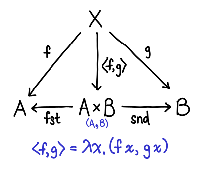
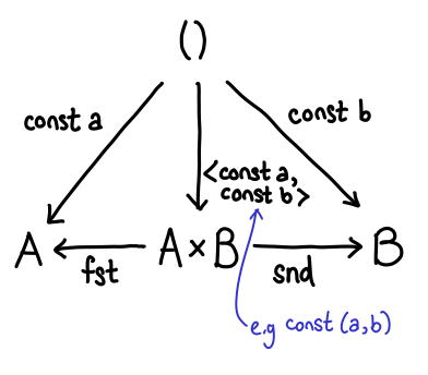
Some of these arrows are pretty easy to explain. What used to be our constructors (Left and Right) are now our destructors (fst and snd). But what of f and g and our new constructor? In fact, \x -> (f x, g x) is in some sense a generalized constructor for pairs, since if we set f = const a and g = const b we can easily get a traditional constructor for a pair (where the specification of the pair itself is the arrow—a little surprising, when you first see it):
So, sums and products are dual to each other. For this reason, sums are often called coproducts.
(Keen readers may have noticed that this presentation is backwards. This is mostly to avoid introducing \x -> (f x, g x), which seemingly comes out of nowhere.)
The unit type (referred to as top) and the bottom type (with no inhabitants) exhibit a duality between one another. We can see this as follows: for any Haskell type, I can trivially construct a function which takes a value of that type and produces unit; it’s const ():
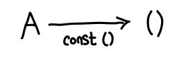
Furthermore, ignoring laziness, this is the only function which does this trick: it’s unique. Let’s flip these arrows around: does there exist a type A for which for any type B, there exists a function A -> B? At first glance, this would seem impossible. B could be anything, including an uninhabited type, in which case we’d be hard pressed to produce anything of the appropriate value. But wait: if A is uninhabited, then I don’t have to do anything: it’s impossible for the function to be invoked!
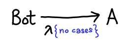
Thus, top and bottom are dual to one another. In fact, they correspond to the concepts of a terminal object and an initial object (respectively) in the category Hask.
One important note about terminal objects: is Int a terminal object? It is certainly true that there are functions which have the type forall a. a -> Int (e.g. const 2). However, this function is not unique: there’s const 0, const 1, etc. So Int is not terminal. For good reason too: there is an easy to prove theorem that states that all terminal objects are isomorphic to one another (dualized: all initial objects are isomorphic to one another), and Int and () are very obviously not isomorphic!
One of the most important components of a functional programming language is the recursive data structure (also known as the inductive data structure). There are many ways to operate on this data, but one of the simplest and most well studied is the fold, possibly the simplest form a recursion one can use.
The diagram for a fold is a bit involved, so we’ll derive it from scratch by thinking about the most common fold known to functional programmers, the fold on lists:
data List a = Cons a (List a) | Nil
foldr :: (a -> r -> r) -> r -> List a -> r
The first two arguments “define” the fold, while the third argument simply provides the list to actually fold over. We could try to draw a diagram immediately:
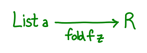
But we run into a little bit of trouble: our diagram is a bit boring, mostly because the pair (a -> r -> r, r) doesn’t really have any good interpretation as an arrow. So what are we to do? What we’d really like is a single function which encodes all of the information that our pair originally encoded.
Well, here’s one: g :: Maybe (a, r) -> r. Supposing we originally had the pair (f, z), then define g to be the following:
g (Just (x, xs)) = f x xs
g Nothing = z
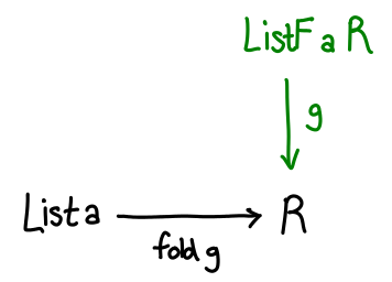
Intuitively, we’ve jammed the folding function and the initial value into one function by replacing the input argument with a sum type. To run f, we pass a Just; to get z, we pass a Nothing. Generalizing a bit, any fold function can be specified with a function g :: F a r -> r, where F a is a functor suitable for the data type in question (in the case of lists, type F a r = Maybe (a, r).) We reused Maybe so that we didn’t have to define a new data type, but we can rename Just and Nothing a little more suggestively, as data ListF a r = ConsF a r | NilF. Compared to our original List definition (Cons a (List a) | Nil), it’s identical, but with all the recursive occurrences of List a replaced with r.
With this definition in hand, we can build out our diagram a bit more:
The last step is to somehow relate List a and ListF a r. Remember how ListF looks a lot like List, just with r replacing List a. So what if we had ListF a (List a)—literally substituting List a back into the functor. We’d expect this to be related to List a, and indeed there’s a simple, unique function which converts one to the other:
in :: ListF a (List a) -> List a
in (ConsF x xs) = Cons x xs
in NilF = Nil
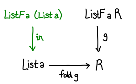
There’s one last piece to the puzzle: how do we convert from ListF a (List a) to ListF a r? Well, we already have a function fold g :: List a -> r, so all we need to do is lift it up with fmap.
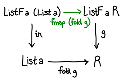
We have a commuting diagram, and require that g . fmap (fold g) = fold g . in.
All that’s left now is to generalize. In general, ListF and List are related using little trick called the Mu operator, defined data Mu f = Mu (f (Mu f)). Mu (ListF a) is isomorphic to List a; intuitively, it replaces all instances of r with the data structure you are defining. So in general, the diagram looks like this:

Now that all of these preliminaries are out of the way, let’s dualize!
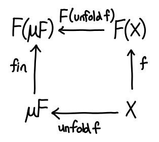
If we take a peek at the definition of unfold in Prelude: unfold :: (b -> Maybe (a, b)) -> b -> [a]; the Maybe (a, b) is exactly our ListF!
The story here is quite similar to the story of sums and products: in the recursive world, we were primarily concerned with how to destruct data. In the corecursive world, we are primarily concerned with how to construct data: g :: r -> F r, which now tells us how to go from r into a larger Mu F.
Dualization is an elegant mathematical concept which shows up everywhere, once you know where to look for it! Furthermore, it is quite nice from the perspective of a category theorist, because when you know two concepts are dual, all the theorems you have on one side flip over to the other side, for free! (This is because all of the fundamental concepts in category theory can be dualized.) If you’re interested in finding out more, I recommend Dan Piponi’s article on data and codata.
October 16, 2012This post is adapted from the talk which Deian Stefan gave for Hails at OSDI 2012.
It is a truth universally acknowledged that any website (e.g. Facebook) is in want of a web platform (e.g. the Facebook API). Web platforms are awesome, because they allow third-party developers to build apps which operate on our personal data.
But web platforms are also scary. After all, they allow third-party developers to build apps which operate on our personal data. For all we know, they could be selling our email addresses to spamlords or snooping on our personal messages. With the ubiquity of third-party applications, it’s nearly trivial to steal personal data. Even if we assumed that all developers had our best interests at heart, we’d still have to worry about developers who don’t understand (or care about) security.
When these third-party applications live on untrusted servers, there is nothing we can do: once the information is released, the third-party is free to do whatever they want. To mitigate this, platforms like Facebook employ a CYA (“Cover Your Ass”) approach:

The thesis of the Hails project is that we can do better. Here is how:
First, third-party apps must be hosted on a trusted runtime, so that we can enforce security policies in software. At minimum, this means we need a mechanism for running untrusted code and expose trusted APIs for things like database access. Hails uses Safe Haskell to implement and enforce such an API.
Next, we need a way of specifying security policies in our trusted runtime. Hails observes that most data models have ownership information built into the objects in question. So a policy can be represented as a function on a document to a set of labels of who can read and a set of labels of who can write. For example, the policy “only Jen’s friends may see her email addresses” is a function which takes the a document representing a user, and returns the “friends” field of the document as the set of valid readers. We call this the MP of an application, since it combines both a model and a policy, and we provide a DSL for specifying policies. Policies tend to be quite concise, and more importantly are centralized in one place, as opposed to many conditionals strewn throughout a codebase.
Finally, we need a way of enforcing these security policies, even when untrusted code is being run. Hails achieves this by implementing thread-level dynamic information flow control, taking advantage of Haskell’s programmable semicolon to track and enforce information flow. If a third-party application attempts to share some data with Bob, but the data is not labeled as readable by Bob, the runtime will raise an exception. This functionality is called LIO (Labelled IO), and is built on top of Safe Haskell.
Third-party applications run on top of these three mechanisms, implementing the view and controller (VC) components of a web application. These components are completely untrusted: even if they have security vulnerabilities or are malicious, the runtime will prevent them from leaking private information. You don’t have to think about security at all! This makes our system a good choice even for implementing official VCs.
One of the example applications we developed was GitStar, a website which hosts Git projects in much the same way as GitHub. The key difference is that almost all of the functionality in GitStar is implemented in third party apps, including project and user management, code viewing and the wiki. GitStar simply provides MPs (model-policy) for projects and users. The rest of the components are untrusted.
Current web platforms make users decide between functionality and privacy. Hails lets you have your cake and eat it too. Hails is mature enough to be used in a real system; check it out at http://www.gitstar.com/scs/hails or just cabal install hails.
October 15, 2012So you’re half bored to death working on your propositional logic problem set (after all, you know what AND and OR are, being a computer scientist), and suddenly the problem set gives you a real stinker of a question:
Is it true that Γ ⊢ A implies that Γ ⊢ ¬A is false?
and you think, “Double negation, no problem!” and say “Of course!” Which, of course, is wrong: right after you turn it in, you think, “Aw crap, if Γ contains a contradiction, then I can prove both A and ¬A.” And then you wonder, “Well crap, I have no intuition for this shit at all.”
Actually, you probably already have a fine intuition for this sort of question, you just don’t know it yet.
The first thing we want to do is establish a visual language for sentences of propositional logic. When we talk about a propositional sentence such as A ∨ B, there are some number of propositional variables which need assignments given to them, e.g. A is true, B is false. We can think of these assignments as forming a set of size 2^n, where n is the number of propositional variables being considered. If n were small, we could simply draw a Venn diagram, but since n could be quite big we’ll just visualize it as a circle:
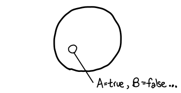
We’re interested in subsets of assignments. There are lots of ways to define these subsets; for example, we might consider the set of assignments where A is assigned to be true. But we’ll be interested in one particular type of subset: in particular, the subset of assignments which make some propositional sentence true. For example, “A ∨ B” corresponds to the set {A=true B=true, A=true B=false, A=false B=true}. We’ll draw a subset graphically like this:
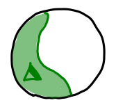
Logical connectives correspond directly to set operations: in particular, conjunction (AND ∧) corresponds to set intersection (∩) and disjunction (OR ∨) corresponds to set union (∪). Notice how the corresponding operators look very similar: this is not by accident! (When I was first learning my logical operators, this is how I kept them straight: U is for union, and it all falls out from there.)

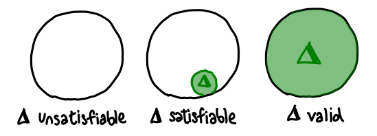
Now we can get to the meat of the matter: statements such as unsatisfiability, satisfiability and validity (or tautology) are simply statements about the shape of these subsets. We can represent each of these visually: they correspond to empty, non-empty and complete subsets respectively:
This is all quite nice, but we haven’t talked about how the turnstile (⊢) aka logical entailment fits into the picture. In fact, when I say something like “B ∨ ¬B is valid”, what I’m actually saying is “⊢ B ∨ ¬B is true”; that is to say, I can always prove “B ∨ ¬B”, no matter what hypothesis I am permitted.”
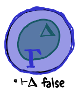
So the big question is this: what happens when I add some hypotheses to the mix? If we think about what is happening here, when I add a hypothesis, I make life “easier” for myself in some sense: the more hypotheses I add, the more propositional sentences are true. To flip it on its head, the more hypotheses I add, the smaller the space of assignments I have to worry about:
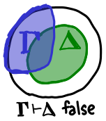
All I need for Γ ⊢ φ to be true is for all of the assignments in Γ to cause φ to be true, i.e. Γ must be contained within φ.

Sweet! So let’s look at this question again:
Is it true that Γ ⊢ A implies that Γ ⊢ ¬A is false?
Recast as a set theory question, this is:
For all Γ and A, is it true that Γ ⊂ A implies that Γ ⊄ A^c? (set complement)
We consider this for a little bit, and realize: “No! For it is true that the empty set is a subset of all sets!” And of course, the empty set is precisely a contradiction: subset of everything (ex falso), and superset of nothing but itself (only contradiction implies contradiction).
It turns out that Γ is a set as well, and one may be tempted to ask whether or not set operations on Γ have any relationship to the set operations in our set-theoretic model. It is quite tempting, because unioning together Γ seems to work quite well: Γ ∪ Δ seems to give us the conjunction of Γ and Δ (if we interpret the sets by ANDing all of their elements together.) But in the end, the best answer to give is “No”. In particular, set intersection on Γ is incoherent: what should {A} ∩ {A ∧ A} be? A strictly syntactic comparison would say {}, even though clearly A ∧ A = A. Really, the right thing to do here is to perform a disjunction, but this requires us to say {A} ∩ {B} = {A ∨ B}, which is confusing and better left out of sight and out of mind.
October 12, 2012Jon Howell dreams of a new Internet. In this new Internet, cross-browser compatibility checking is a distant memory and new features can be unilaterally be added to browsers without having to convince the world to upgrade first. The idea which makes this Internet possible is so crazy, it just might work.
What if a web request didn’t just download a web page, but the browser too?
“That’s stupid,” you might say, “No way I’m running random binaries from the Internet!” But you’d be wrong: Howell knows how to do this, and furthermore, how to do so in a way that is safer than the JavaScript your browser regularly receives and executes. The idea is simple: the code you’re executing (be it native, bytecode or text) is not important, rather, it is the system API exposed to the code that determines the safety of the system.
Consider today’s browser, one of the most complicated pieces of software installed on your computer. It provides interfaces to “HTTP, MIME, HTML, DOM, CSS, JavaScript, JPG, PNG, Java, Flash, Silverlight, SVG, Canvas, and more”, all of which almost assuredly have bugs. The richness of the APIs are their own downfall, as far as security is concerned. Now consider what APIs a native client would need to expose, assuming that the website provided the browser and all of the libraries.
The answer is very little: all you need is a native execution environment, a minimal interface for persistent state, an interface for external network communication and an interface for drawing pixels on the screen (ala VNC). That’s it: everything else can be implemented as untrusted native code provided by the website. This is an interface that is small enough that we would have a hope of making sure that it is bug free.
What you gain from this radical departure from the original Internet is fine-grained control over all aspects of the application stack. Websites can write the equivalents of native apps (ala an App Store), but without the need to press the install button. Because you control the stack, you no longer need to work around browser bugs or missing features; just pick an engine that suits your needs. If you need push notifications, no need to hack it up with a poll loop, just implement it properly. Web standards continue to exist, but no longer represent a contract between website developers and users (who couldn’t care less about under the hood); they are simply a contract between developers and other developers of web crawlers, etc.
Jon Howell and his team have implemented a prototype of this system, and you can read more about the (many) technical difficulties faced with implementing a system like this. (Do I have to download the browser every time? How do I implement a Facebook Like button? What about browser history? Isn’t Google Native Client this already? Won’t this be slow?)
As a developer, I long for this new Internet. Never again would I have to write JavaScript or worry browser incompatibilities. I could manage my client software stack the same way I manage my server software stack, and use off-the-shelf components except in specific cases where custom software was necessary.) As a client, my feelings are more ambivalent. I can’t use Adblock or Greasemonkey anymore (that would involve injecting code into arbitrary executables), and it’s much harder for me to take websites and use them in ways their owners didn’t originally expect. (Would search engines exist in the same form in this new world order?) Oh brave new world, that has such apps in’t!
October 3, 2012Caveat emptor: half-baked research ideas ahead.
What is a monad? One answer is that it is a way of sequencing actions in a non-strict language, a way of saying “this should be executed before that.” But another answer is that it is programmable semicolon, a way of implementing custom side-effects when doing computation. These include bread and butter effects like state, control flow and nondeterminism, to more exotic ones such as labeled IO. Such functionality is useful, even if you don’t need monads for sequencing!
Let’s flip this on its head: what does a programmable semicolon look like for a call-by-need language? That is, can we get this extensibility without sequencing our computation?
At first glance, the answer is no. Most call-by-value languages are unable to resist the siren’s song of side effects, but in call-by-need side effects are sufficiently painful that Haskell has managed to avoid them (for the most part!) Anyone who has worked with unsafePerformIO with NOINLINE pragma can attest to this: depending on optimizations, the effect may be performed once, or it may be performed many times! As Paul Levy says, “A third method of evaluation, call-by-need, is useful for implementation purposes. but it lacks a clean denotational semantics—at least for effects other than divergence and erratic choice whose special properties are exploited in [Hen80] to provide a call-by-need model. So we shall not consider call-by-need.” Paul Levy is not saying that for pure call-by-need, there are no denotational semantics (these semantics coincide exactly with call-by-name, call-by-need’s non-memoizing cousin), but that when you add side-effects, things go out the kazoo.
But there’s a hint of an angle of attack here: Levy goes on to show how to discuss side effects in call-by-name, and has no trouble specifying the denotational semantics here. Intuitively, the reason for this is that in call-by-name, all uses (e.g. case-matches) on lazy values with an effect attached cause the effect to manifest. Some effects may be dropped (on account of their values never being used), but otherwise, the occurrence of effects is completely deterministic.
Hmm!
Of course, we could easily achieve this by giving up memoization, but that is a bitter pill to swallow. So our new problem is this: How can we recover effectful call-by-name semantics while preserving sharing?
In the case of the Writer monad, we can do this with all of the original sharing. The procedure is very simple: every thunk a now has type (w, a) (for some fixed monoidal w). This tuple can be shared just as the original a was shared, but now it also has an effect w embedded with it. Whenever a would be forced, we simply append effect to the w of the resulting thunk. Here is a simple interpreter which implements this:
{-# LANGUAGE GADTs #-}
import Control.Monad.Writer

data Expr a where
    Abs :: (Expr a -> Expr b) -> Expr (a -> b)
    App :: Expr (a -> b) -> Expr a -> Expr b
    Int :: Int -> Expr Int
    Add :: Expr Int -> Expr Int -> Expr Int
    Print :: String -> Expr a -> Expr a

instance Show (Expr a) where
    show (Abs _) = "Abs"
    show (App _ _) = "App"
    show (Int i) = show i
    show (Add _ _) = "Add"
    show (Print _ _) = "Print"

type M a = Writer String a
cbneed :: Expr a -> M (Expr a)
cbneed e@(Abs _) = return e
cbneed (App (Abs f) e) =
    let ~(x,w) = run (cbneed e)
    in cbneed (f (Print w x))
cbneed e@(Int _) = return e
cbneed (Add e1 e2) = do
    Int e1' <- cbneed e1
    Int e2' <- cbneed e2
    return (Int (e1' + e2'))
cbneed (Print s e) = do
    tell s
    cbneed e

sample = App (Abs (\x -> Print "1" (Add x x))) (Add (Print "2" (Int 2)) (Int 3))
run = runWriter
Though the final print out is "122" (the two shows up twice), the actual addition of 2 to 3 only occurs once (which you should feel free to verify by adding an appropriate tracing call). You can do something similar for Maybe, by cheating a little: since in the case of Nothing we have no value for x, we offer bottom instead. We will never get called out on it, since we always short-circuit before anyone gets to the value.
There is a resemblance here to applicative functors, except that we require even more stringent conditions: not only is the control flow of the computation required to be fixed, but the value of the computation must be fixed too! It should be pretty clear that we won’t be able to do this for most monads. Yesterday on Twitter, I proposed the following signature and law (reminiscent of inverses), which would need to be implementable by any monad you would want to do this procedure on (actually, you don’t even need a monad; a functor will do):
extract :: Functor f => f a -> (a, f ())
s.t.  m == let (x,y) = extract m in fmap (const x) y
but it seemed only Writer had the proper structure to pull this off properly (being both a monad and a comonad). This is a shame, because the application I had in mind for this bit of theorizing needs the ability to allocate cells.
Not all is lost, however. Even if full sharing is not possible, you might be able to pull off partial sharing: a sort of bastard mix of full laziness and partial evaluation. Unfortunately, this would require substantial and invasive changes to your runtime (and I am not sure how you would do it if you wanted to CPS your code), and so at this point I put away the problem, and wrote up this blog post instead.
September 28, 2012There is a bit of scaffolding involved with making Core-to-Core transforming GHC plugins, so I made a little project, based off of Max Bolingbroke’s examples, which is a nice, clean template project which you can use to create your own GHC plugins. In particular, it has documentation and pointers to the GHC source as well as a handy-dandy shell script rename.sh MyProjectName which will let you easily rename the template project into whatever name you want. You can find it on GitHub. I’ll probably be adding more to it as I go along; let me know about any bugs too.
September 24, 2012Done. This adjective rarely describes any sort of software project—there are always more bugs to fix, more features to add. But on September 20th, early one afternoon in France, Georges Gonthier did just that: he slotted in the last component of a six year project, with the laconic commit message, “This is really the End.”
It was complete: the formalization of the Feit-Thompson theorem.
If you’re not following the developments in interactive theorem proving or the formalization of mathematics, this achievement may leave you scratching your head a little. What is the Feit-Thompson theorem? What does it mean for it to have been formalized? What was the point of this exercise? Unlike the four coloring theorem which Gonthier and his team tackled previously in 2005, the Feit-Thompson theorem (also known as the odd order theorem) is not easily understandable by non-mathematician without a background in group theory (I shall not attempt to explain it). Nor are there many working mathematicians whose lives will be materially impacted by the formalization of this particular theorem. But there is a point; one that can be found between the broad motivation behind the computer-assisted theorem proving and the fascinating social context surrounding the Feit-Thompson theorem.
While the original vision of automated theorem proving, articulated by David Hilbert, was one where computers completely replaced mathematicians in the work of proving theorems (mathematicians would be consigned to dreaming up interesting theorem statements to prove), modern researchers in the formalization of mathematics consider the more modest question of whether or not a proof is true. That is to say, humans are fallible and can make mistakes while reviewing the proofs of their colleagues, while the computer is an idiot-savant who, once spoon-fed the contents of a proof, is essentially infallible in its judgment of correctness. The proofs of undergraduate mathematics classes don’t really need this treatment (after all, they have been inflicted on countless math majors over the centuries), but there are a few areas where this extra boost of confidence is really appreciated:
- In theorems which are found in conventional software systems, due to the large number of incidental details making proofs superficial but large,
- In extremely tricky, consistently unintuitive areas of mathematics, including questions of provability and soundness, and
- In extremely long and involved proofs, for which traditional verification by human mathematicians is a Herculean task.
It is in this last area that we can really place both the Four Color Theorem and the Feit-Thompson Theorem. The Four Color Theorem’s original proof was controversial because of its reliance on a computer to solve 1936 special cases which the proof depended on. The Feit-Thompson Theorem is a bit of an annoyance to many mathematicians, due to its length: 255 pages, the global structure of which has resisted over half a century of attempts at simplification. And it itself is just a foothill on the way to the monster theorem that is the classification of finite simple groups (comprising tens of thousands of pages of proof.)
Formalizing the entirety of the Feit-Thompson is a technical achievement which applies computer-assisted theorem proving to a tremendously nontrivial mathematical proof, and does so in a setting where the ability to state “Feit-Thompson is True” has non-zero information content. It demonstrates that theorem proving in Coq does scale (at least, well enough pull off a proof of this scale) and it has generated a large toolbox for handling features of real mathematics including heavily overloaded notation and handing the composition of many, disparate theories (all of which the proof draws upon).
Of course, there is one niggling concern: what if there is a bug, and what Gonthier and his team have proved is not actually the Feit-Thompson Theorem? A story I once heard while I was at Galois was of a research intern who had been tasked with proving some theorems. He had some trouble at first, but eventually pulled off the first theorem and moved to the next, gradually gaining speed. Eventually, his advisor took a look at these proofs and realized that he had been taking advantage of a soundness problem in the proof checker to solve the proofs. I wonder if this is a story that wizened PhD students tell the first years to give them nightmares.
But I think the risk of this is very low. The mechanized proof follows the original quite closely, and so a wrong definition or a soundness bug is likely only to pose a local problem for the proof that can be easily solved. Indeed, if there is a problem with the proof that is so great that the proof must be thrown out and done again, that would be very interesting—it would say something about the original proof as well. That would be surprising, and worthy of attention, for it could mean the end of the proof of the Feit-Thompson Theorem as we know it. But I don’t think we live in that world.
Pop the champagne, and congratulations to Gonthier and his team!
September 17, 2012Safe Haskell is a new language pragma for GHC which allows you to run untrusted code on top of a trusted code base. There are some common misconceptions about how Safe Haskell works in practice. In this post, I’d like to help correct some of these misunderstandings.
Although an IO action here is certainly unsafe, it is not rejected by Safe Haskell per se, because the type of this expression clearly expresses the fact that the operation may have arbitrary side effects. Your obligation in the trusted code base is to not run untrusted code in the IO monad! If you need to allow limited input/output, you must define a restricted IO monad, which is described in the manual.
Even with killThread, it is all to easy to permanently tie up a capability by creating a non-allocating infinite loop. This bug has been open for seven years now, but we consider this a major deficiency in Safe Haskell, and are looking for ways to prevent this from occurring. But as things are now, Safe Haskell programs need to be kept under check using operating system level measures, rather than just Haskell’s thread management protocols.
The Trustworthy keyword is used to mark modules which use unsafe language features and/or modules in a “safe” way. The safety of this is vouched for by the maintainer, who inserts this pragma into the top of the module file. Caveat emptor! After all, there is no reason that you should necessarily believe a maintainer who makes such a claim. So, separately, you can trust a package, via the ghc-pkg database or the -trust flag. But GHC also allows you to take the package maintainer at their word, and in fact does so by default; to make it distrustful, you have to pass -fpackage-trust. The upshot is this:
| Module trusted? | (no flags) | -fpackage-trust |
|---|
| Package untrusted | Yes | No |
| Package trusted | Yes | Yes |
If you are serious about using Safe Haskell to run untrusted code, you should always run with -fpackage-trust, and carefully confer trusted status to packages in your database. If you’re just using Safe Haskell as a way of enforcing code style, the default are pretty good.
Safe Haskell offers safety inference, which automatically determines if a module is safe by checking if it would compile with the -XSafe flag. Safe inferred modules can then be freely used by untrusted code. Now, suppose that this module (inferred safe) was actually Data.HTML.Internal, which exported constructors to the inner data type which allowed a user to violate internal invariants of the data structure (e.g. escaping). That doesn’t seem very safe!
The sense in which this is safe is subtle: the correctness of the trusted code base cannot rely on any invariants supplied by the untrusted code. For example, if the untrusted code defines its own buggy implementation of a binary tree, catching the bugginess of the untrusted code is out of scope for Safe Haskell’s mission. But if our TCB expects a properly escaped HTML value with no embedded JavaScript, the violation of encapsulation of this type could mean the untrusted code could inject XSS.
David Terei and I have some ideas for making the expression of trust more flexible with regards to package boundaries, but we still haven’t quite come to agreement on the right design. (Hopefully we will soon!)
Safe Haskell is at its heart a very simple idea, but there are some sharp edges, especially when Safe Haskell asks you to make distinctions that aren’t normally made in Haskell programs. Still, Safe Haskell is rather unique: while there certainly are widely used sandboxed programming languages (Java and JavaScript come to mind), Safe Haskell goes even further, and allows you to specify your own, custom security policies. Combine that with a massive ecosystem of libraries that play well with this feature, and you have a system that you really can’t find anywhere else in the programming languages universe.
September 12, 2012One of the most mind-bending features of the untyped lambda calculus is the fixed-point combinator, which is a function fix with the property that fix f == f (fix f). Writing these combinators requires nothing besides lambdas; one of the most famous of which is the Y combinator λf.(λx.f (x x)) (λx.f (x x)).
Now, if you’re like me, you saw this and tried to implement it in a typed functional programming language like Haskell:
Prelude> let y = \f -> (\x -> f (x x)) (\x -> f (x x))

<interactive>:2:43:
    Occurs check: cannot construct the infinite type: t1 = t1 -> t0
    In the first argument of `x', namely `x'
    In the first argument of `f', namely `(x x)'
    In the expression: f (x x)
Oops! It doesn’t typecheck.
There is a solution floating around, which you might have encountered via a Wikipedia article or Russell O’Connor’s blog, which works by breaking the infinite type by defining a newtype:
Prelude> newtype Rec a = In { out :: Rec a -> a }
Prelude> let y = \f -> (\x -> f (out x x)) (In (\x -> f (out x x)))
Prelude> :t y
y :: (a -> a) -> a
There is something very strange going on here, which Russell alludes to when he refers to Rec as “non-monotonic”. Indeed, any reasonable dependently typed language will reject this definition (here it is in Coq):
Inductive Rec (A : Type) :=
  In : (Rec A -> A) -> Rec A.

(* Error: Non strictly positive occurrence of "Rec" in "(Rec A -> A) -> Rec A". *)
What is a “non strictly positive occurrence”? It is reminiscent to “covariance” and “contravariance” from subtyping, but more stringent (it is strict, after all!) Essentially, a recursive occurrence of the type (e.g. Rec) may not occur to the left of a function arrow of a constructor argument. newtype Rec a = In (Rec a) would have been OK, but Rec a -> a is not. ((Rec a -> a) -> a is not OK either, despite Rec a being in a positive position.)
There are good reasons for rejecting such definitions. The most important of these is excluding the possibility of defining the Y Combinator (party poopers!) which would allow us to create a non-terminating term without explicitly using a fixpoint. This is not a big deal in Haskell (where non-termination abounds), but in a language for theorem proving, everything is expected to be terminating, since non-terminating terms are valid proofs (via the Curry-Howard isomorphism) for any proposition! Thus, adding a way to sneak in non-termination with the Y Combinator would make the type system very unsound. Additionally, there is a sense in which types that are non-strictly positive are “too big”, in that they do not have set theoretic interpretations (a set cannot contain its own powerset, which is essentially what newtype Rec = In (Rec -> Bool) claims).
To conclude, types like newtype Rec a = In { out :: Rec a -> a } look quite innocuous, but they’re actually quite nasty and should be used with some care. This is a bit of a bother for proponents of higher-order abstract syntax (HOAS), who want to write types like:
data Term = Lambda (Term -> Term)
          | App Term Term
Eek! Non-positive occurrence of Term in Lambda strikes again! (One can feel the Pittsburgh-trained type theorists in the audience tensing up.) Fortunately, we have things like parametric higher-order abstract syntax (PHOAS) to save the day. But that’s another post…
Thanks to Adam Chlipala for first introducing me to the positivity condition way back last fall during his Coq class, Conor McBride for making the offhand comment which made me actually understand what was going on here, and Dan Doel for telling me non-strictly positive data types don’t have set theoretic models.