ezyang’s blog

Greetings from 2024! An official pattern matching PEP has been accepted https://peps.python.org/pep-0636/ and is available in Python 3.10. Class patterns are tested using isinstance, with no inheritance structure necessary, making the pattern described in this post 100% forward compatible to real pattern matching.

---

One of the features I miss most in non-Haskell programming languages is algebraic data types (ADT). ADTs fulfill a similar role to objects in other languages, but with more restrictions: objects are an open universe, where clients can implement new subclasses that were not known at definition time; ADTs are a closed universe, where the definition of an ADT specifies precisely all the cases that are possible. We often think of restrictions of a bad thing, but in the case of ADTs, the restriction of being a closed universe makes programs easier to understand (a fixed set of cases to understand, as opposed to a potentially infinite set of cases) and allows for new modes of expression (pattern matching). ADTs make it really easy to accurately model your data structures; they encourage you to go for precise types that make illegal states unrepresentable. Still, it is generally not a good idea to try to manually reimplement your favorite Haskell language feature in every other programming language you use, and so for years I've suffered in Python under the impression that ADTs were a no go.

Recently, however, I have noticed that a number of new features in Python 3 have made it possible to use objects in the same style of ADTs, in idiomatic Python with virtually no boilerplate. The key features:

• A structural static type checking system with mypy; in particular, the ability to declare Union types, which let you represent values that could be one of a fixed set of other types, and the ability to refine the type of a variable by performing an isinstance check on it.
• The dataclasses library, which allows you to conveniently define (possibly immutable) structures of data without having to write boilerplate for the constructor.

The key idea: define each constructor as a dataclass, put the constructors together into an ADT using a Union type, and use isinstance tests to do pattern matching on the result. The result is just as good as an ADT (or better, perhaps; their structural nature bears more similarity to OCaml's polymorphic variants).

Here's how it works. Let's suppose that you want to define an algebraic data type with two results:

data Result
   = OK Int
   | Failure String

showResult :: Result -> String
showResult (OK result) = show result
showResult (Failure msg) = "Failure: " ++ msg

First, we define each constructor as a dataclass:

from dataclasses import dataclass

@dataclass(frozen=True)
class OK:
    result: int

@dataclass(frozen=True)
class Failure:
    msg: str

Using the automatically generated constructors from dataclasses, we can construct values of these dataclasses using OK(2) or Failure("something wrong"). Next, we define a type synonym for the union of these two classes:

Result = Union[OK, Failure]

Finally, we can do pattern matching on Result by doing isinstance tests:

def assert_never(x: NoReturn) -> NoReturn:
    raise AssertionError("Unhandled type: {}".format(type(x).__name__))

def showResult(r: Result) -> str:
    if isinstance(r, OK):
        return str(r.result)
    elif isinstance(r, Failure):
        return "Failure: " + r.msg
    else:
        assert_never(r)

assert_never is a well known trick for doing exhaustiveness checking in mypy. If we haven't covered all cases with enough isinstance checks, mypy will complain that assert_never was given a type like UnhandledCtor when it expected NoReturn (which is the uninhabited type in Python).

That's all there is to it. As an extra bonus, this style of writing unions is compatible with the structured pattern matching PEP, if it actually gets accepted. I've been using this pattern to good effect in our recent rewrite of PyTorch's code generator. If you have the opportunity to work in a statically typed Python codebase, give this style of code a try!

If this is your first time reading about PyTorch internals, you might want to check out my PyTorch internals post first. In this post, I want to talk about one particular part of PyTorch's internals: the dispatcher. At a first glance, the dispatcher is just a glorified if statement: based on some information about the tensor inputs, decide what piece of code should be called. So why should we care about the dispatcher?

Well, in PyTorch, a lot of things go into making an operator work. There is the kernel that does the actual work, of course; but then there is support for reverse mode automatic differentiation, e.g., the bits that make loss.backward() work. Oh, and if your code under torch.jit.trace, you can get a trace of all the operations that were run. Did I mention that if you run these operations on the inside of a vmap call, the batching behavior for the operators is different? There are so many different ways to interpret PyTorch operators differently, and if we tried to handle all of them inside a single function named add, our implementation code would quickly devolve into an unmaintainable mess. The dispatcher is not just an if statement: it is a really important abstraction for how we structure our code internally PyTorch... and it has to do so without degrading the performance of PyTorch (too much, anyway).

At the end of this post, our goal will be to understand all the different parts of this picture fit together. This post will proceed in three parts.

First, we'll talk about the dispatcher itself. What is the dispatcher, how does it decide what kernel to call? Second, we'll talk about the operator registration API, which is the interface by which we register kernels into the dispatcher. Finally, we'll talk about boxing and unboxing, which are a cross-cutting feature in the dispatcher that let you write code once, and then have it work on all kernels.

For the longest time, I thought of implicit parameters and dynamic scoping were basically the same thing, since they both can be used to solve similar problems (e.g., the so called "configuration problem" where you need to plumb down some configuration deep into a nested body of function definitions without defining them all explicitly). But implicit parameters have a reputation of being something you shouldn't use (use reflection instead), whereas dynamic scoping via the reader monad is a useful and well understood construct (except for the bit where you have to monadify everything). Why the difference?

Oleg points out that implicit parameters are not really dynamic scoping, and gives an example where Lisp and Haskell disagree. And you don't even want the Lisp behavior in Haskell: if you think about the operational notion of dynamic scoping (walk up the stack until you find a binding site of the dynamic variable), it's not very compatible with laziness, since a thunk (which accesses a dynamic variable) will be forced at some unpredictable point in program execution. You really don't want to have to reason about where exactly a thunk will be executed to know how its dynamic variables will be bound, that way lies madness. But somehow, in a strict language, no one has trouble figuring out what should happen with dynamic scoping (well, mostly--more on this shortly).

It turns out that the research community has figured out the difference is that implicit parameters are a coeffect. I believe this was first observed in Coeffects: Unified static analysis of context-dependence (a more modern presentation is in Coeffects: A calculus of context-dependent computation; and a more Haskelly presentation can be found in Embedding effect systems in Haskell). Although, Tomas was commenting on my blog in 2012 about similar ideas, so this probably had been in the works for a while. The key point is that for some coeffects (namely, implicit parameters), call-by-name reduction preserves types and coeffects, and so implicit parameters do not blow up in your face in the same way dynamic scoping (an effect) would. These necessarily behave differently! Type classes are coeffects too, and this is why modern use of implicit parameters in Haskell explicitly acknowledges this (e.g., in the reflection package).

At this year's ICFP, I was pointed at an interesting technical report about implicit values and functions in Koka, a new twist on the dynamic scoping. I found myself wondering if Haskell implicit parameters could learn a thing or two from this work. Implicit values make the good choice of defining implicit values globally at the top level, so that they can participate in normal module namespacing, as opposed to an un-namespaced bag of dynamically scoped names (this is also an improvement that reflection makes over implicit parameters). But actually, it seems to me that implicit functions are taking a page from implicit parameters!

The big innovation is the implicit function is that it resolves all dynamic references in the function (not just lexically, but for all further dynamic calls) to the lexical scope (the dynamic scope at the time the function was defined), producing a function that has no dependence on implicit values (aka, has no effect saying that the implicit value must be defined at the time the function is called.) This is exactly what an implicit parameter let ?x = ... binding would have done, in effect directly filling in the dictionary for the implicit function at definition site, rather than waiting. Very contextual! (Of course, Koka implements this using algebraic effects, and gets to the right semantics with a very simple translation anyway). The result is not exactly dynamic scoping, but as the TR says, it leads to better abstraction.

It is difficult to see how implicit values/functions could make their way back into Haskell, at least without some sequencing constructing (e.g., a monad) lurking around. Though implicit functions behave much like implicit parameters, the rest of the dynamic scoping (including the binding of the implicit function itself) is just good old effectful (not coeffectful) dynamic scope. And you can't just do that in Haskell, without breaking type preservation under beta-reduction and eta-expansion. Haskell has no choice but to go all the way, and once you get beyond the obvious problems of implicit parameters (which reflection fixes), things seem to mostly work out.

I've recently been working on a revamp of how we specify tensor shape formulas in PyTorch. As part of this process, I classified every single operator in PyTorch by its shaping behavior; yes, that's all 1364 of them (this includes each variant of an operator; e.g., inplace and out= keyword variants). During the process, I tried to come up with categories to help classify what operators did. One of the surprises from the process was discovering that shaping behaviors that I previously thought were uncommon, actually showed up a bit more often than one might have expected.

These categories are interesting in their own right and can be used to help understand how PyTorch's API fits together. Here are all the categories I devised.

TensorIterator (505, e.g., add, sum) operators are PyTorch's bread and butter; these operators do pointwise operations and reductions and support broadcasting and type promotion. The name TensorIterator refers to an internal abstraction we have in PyTorch for implementing these operations; you can read more about it on the wiki and in this blog post. TensorIterator is a real workhorse in PyTorch: the plurarity (though not majority) of operators are implemented in this way! Note that this category includes some functions that used equivalent, legacy functionality (but did not exactly use TensorIterator).

Fixed (273, e.g., convolution, addbmm) operators are operators which only work on a fixed number of dimensions. This assumption makes writing efficient kernels a lot easier, as indexing math is simple with fixed dimensionality. (For example, TensorAccessor is an internal class which lets you view a tensor at fixed dimensionality known at compile time). Sometimes, the first dimension is treated as a batch dimension, but not always (unfortunately, I didn't distinguish these cases in my dataset). Some fixed operators actually support multiple dimensions, but only a fixed number of them; for example, because we only support 1-3D convolutions, this counts as fixed. (Compare with this FeatureBatched, below!)

N-Dimensional (107, e.g., squeeze, index_add, tensordot) operators are operators which work generically on tensors of arbitrary dimensionality. These are the operations for which it is difficult to write generic shaping rules for in symbolic form, as you need a language that can talk about list manipulations. An important subclass of N-dimensional operators are Identity (42, e.g., clone, contiguous; not included in the count above) operators work over arbitrary dimensionality, but they always return a tensor with the same size as their input. Another subclass are Flatten (11, e.g. take, bucketize) operators which accept tensors of any dimensionality, but always treat them as 1D tensors internally.

Composite (95, e.g., kl_div, isfinite) operators are implemented in other operators, and don't themselves have shape checking (instead, they rely on the operations they call to check shapes). Note this category is probably a bit underreported, as in some cases when it was obvious what the underlying behavior of an operator was, I classified the operator as that category, rather than Composite.

Batched (94, e.g., nll_loss, adaptive_avg_pool2d) operators are like fixed dimensionality operators, except they accept an arbitrary number of batch dimensions at their beginning. Many fixed operators should be batched operators; others cannot be converted into batched operators without introducing ambiguity as to where the batch dimensions end. Compare these with FeatureBatched (19, e.g., batch_norm, embedding) operators, which are like batched operators, but rather than accept batch dimensions at the beginning, they accept an arbitrary number of feature dimensions at the end.

Factory (90, e.g., empty) operators produce new tensors without having any tensor inputs.

Trivial (59, e.g., size, is_floating_point) operators aren't actual tensor operations, but ways to return non-Tensor information or access internal data structures

Sparse (40) operators are special because their size calculations take account of both dense and sparse dimensions.

Dynamic (15, e.g., unique) operators produce outputs whose shapes depend on the data of their input tensors

Variadic (14, e.g., cat) operators take multiple input tensors; similar to n-dimensional operations they are difficult to capture symbolic

You can take a look at the full data set at https://docs.google.com/spreadsheets/d/e/2PACX-1vQQFW0T_bucT5KZn0BHYTC1KYhkL6ZMG5ZxQWc6UmAkHUDYpqkpzXnsb59uv2TB0Jgc1Q6qO63bx6WQ/pubhtml

vmap is an interface popularized by JAX which offers you a vectorizing map. Semantically, a vmap is exactly equivalent to a map in Haskell; the key difference is that operations run under a vmap are vectorized. If you map a convolution and a matrix multiply, you will have one big loop which repeatedly calls convolution and matrix multiply for each entry in your batch. If you vmap a convolution and matrix multiply, you'll call the batched versions of convolution and matrix multiply once. Unless you have a fuser, on most modern deep learning frameworks, calling the batched implementations of these operations will be much faster.

JAX implements vmap in a somewhat complicated fashion; they have a "batched interpreter" which translates operations on primitives into their batched versions, and have to track metadata about what tensors are batched and in what way so that they can insert appropriate broadcasts and unsqueezes. I mentioned this to Simon Peyton Jones, and he immediately asked, couldn't Haskell's typechecker work this out automatically? The answer is, yes! All of the book-keeping JAX has to do is effectively doing runtime type inference; if you have a compiler that can do it for you at compile time, there is nearly nothing to implement.

To give away the punchline, we are going to implement a family of functions vmap that will run these two examples:

example1 :: [Float] -> [Float] -> [Float]
example1 a0 b0 =
  vmap0_2 (\a b -> add a b) a0 b0

example2 :: [Float] -> [Float] -> [[Float]]
example2 a0 b0 =
  vmap0 (\a -> vmap1 (\b -> add a b) b0) a0

When run in an interpreter, we will see:

*Test> example1 [1,2,3] [4,6,8]
[5.0,8.0,11.0]
*Test> example2 [1,2,3] [4,6,8]
[[5.0,7.0,9.0],[6.0,8.0,10.0],[7.0,9.0,11.0]]

These results are equivalent to what you would have gotten using a plain old map; however, there will be no loop in the implementation of vmap. (The fact that we can't write a single vmap that works universally is due to a limitation in Haskell; we'll discuss this more later.)

---

We're going to need a few language extensions, so let's get this out of the way first:

{-# LANGUAGE RankNTypes, GADTs, MultiParamTypeClasses,
             KindSignatures, TypeApplications, FunctionalDependencies,
             FlexibleContexts, FlexibleInstances, UndecidableInstances,
             IncoherentInstances #-}

Our plan of attack is that we want to write the definitions of vmap so that we infer a type for add which makes the necessary broadcasting clear. A trivial implementation of vmap would have the signature ([a] -> [b]) -> [a] -> [b] (aka the identity function), but the standard list type doesn't let us distinguish between dimensions we should broadcast together, and dimensions we shouldn't (this is the reason example1 and example2 give different results: in example2, we broadcast along each dimension separately, so that we end up with a cartesian product in the end; in example1, we broadcast the dimensions together and get the zippy behavior). Each distinct invocation of vmap should give us a new dimension, which ought not to be mixed up with other invocations of vmap. When you hear this in Haskell, your first instinct should be, "I know, let's use a rank 2 type!" vmap moves us from the non-type-branded world of vanilla lists [Float] to a type-branded world of size-indexed vectors Vec s Float, where the s variables are all skolem variables bound by our rank 2 type:

data Vec s a = Vec { unVec :: [a] }
instance Functor (Vec s) where
  fmap f (Vec xs) = Vec (map f xs)

vmap0 :: (forall s. Vec s a -> Vec s b) -> [a] -> [b]
vmap0 f = unVec . f . Vec

The implementation of vmap0 doesn't do anything: we just wrap the lists into their type-branded equivalent vectors. We can also provide a 2-ary version of vmap0, which takes two lists and assigns them the same type branding all at once:

vmap0_2 :: (forall s. Vec s a -> Vec s b -> Vec s c) -> [a] -> [b] -> [c]
vmap0_2 f a b = unVec (f (Vec a) (Vec b))

(In principle, some sort of applicative-y thing should make it possible to write just a vap (analogous to ap) and then get all of the n-ary versions for free, but in my brief investigation I didn't see a good way of doing this.)

When we nest vmap, it may be the case that the function doesn't directly return a Vec s b, but a functor containing Vec s b. vmap1 handles this case (we'll discuss this more shortly):

vmap1 :: Functor f => (forall s. Vec s a -> f (Vec s b)) -> [a] -> f [b]
vmap1 f = fmap unVec . f . Vec

With our implementations of vmap in hand, we can take a look at our examples and ask Haskell what the type of add ought to be, if we didn't have an implementation of it:

example1 :: [Float] -> [Float] -> [Float]
example1 a0 b0 =
  vmap0_2 (\a b -> _add a b) a0 b0

Gives:

• Found hole: _add :: Vec s Float -> Vec s Float -> Vec s Float
  Where: ‘s’ is a rigid type variable bound by
           a type expected by the context:
             forall s. Vec s Float -> Vec s Float -> Vec s Float

However:

example2 :: [Float] -> [Float] -> [[Float]]
example2 a0 b0 =
  vmap0 (\a -> vmap1 (\b -> _add a b) b0) a0

Gives:

• Found hole:
    _add :: Vec s Float -> Vec s1 Float -> Vec s (Vec s1 Float)
  Where: ‘s1’ is a rigid type variable bound by
           a type expected by the context:
             forall s1. Vec s1 Float -> Vec s (Vec s1 Float)
           at test.hs:41:20-44
         ‘s’ is a rigid type variable bound by
           a type expected by the context:
             forall s. Vec s Float -> Vec s [Float]
           at test.hs:41:7-48

Notice that the inferred types of _add are different in these two cases: in the first example, we infer that we have two tensors batched in the same way, and we want to "zip" them together. In the second example, we see that each tensor has a distinct batch dimension, and we end up with a 2-D result!

At this point, the job of vmap is done: our holes have types which we can use to determine what the necessary behavior is. You could use these types to select an appropriate kernel to perform vectorized addition. But I promised runnable code, so let's implement a simple version of add using old fashioned map.

The good old fashioned way to do type level computation in Haskell is with a type class, of course! Let's define a multi-parameter type class for the function add; unlike the definition of (+) in Num, we'll let the inputs and output all have different types:

class Add a b c | a b -> c where
  add :: a -> b -> c

We can easily implement addition on plain floating point:

instance Add Float Float Float where
  add = (+)

If I pass add two arguments whose outer-most vector agree in their type brand (aka, they came from the same vmap), I should zip them together, as I did in example1. I can write another instance to express this logic:

instance Add a b r  => Add (Vec s a) (Vec s b) (Vec s r) where
  add (Vec a) (Vec b) = Vec (zipWith add a b)

Otherwise, I should broadcast one of the dimensions and then do an addition on the inside. This choice can't easily be made locally, so I have to define these two incoherent instances:

instance Add a b r => Add (Vec s a) b (Vec s r) where
  add (Vec a) b = Vec (map (\x -> add x b) a)

instance Add a b r => Add a (Vec s b) (Vec s r) where
  add a (Vec b) = Vec (map (\x -> add a x) b)

(GHC's type class resolution engine doesn't backtrack, so I'm not actually sure how it manages to pick the correct instance to use, but in my testing, I got the right instance no matter what order I specified the arguments to add.)

That's it! Running the two examples:

example1 :: [Float] -> [Float] -> [Float]
example1 a0 b0 =
  vmap0_2 (\a b -> add a b) a0 b0

example2 :: [Float] -> [Float] -> [[Float]]
example2 a0 b0 =
  vmap0 (\a -> vmap1 (\b -> add a b) b0) a0

I get:

*Test> example1 [1,2,3] [4,6,8]
[5.0,8.0,11.0]
*Test> example2 [1,2,3] [4,6,8]
[[5.0,7.0,9.0],[6.0,8.0,10.0],[7.0,9.0,11.0]]

---

So there you have it! vmap in less than a dozen lines of Haskell. One unsatisfactory thing about this implementation is the necessity to define vmap0, vmap1, etc. Can't we just define a generic vmapG ::  (forall s. Vec s a -> f (Vec s b)) -> [a] -> f [b] and have f unify with, well, the identity type lambda /\a. a when we need it to have the type of vmap0? Regretfully, type inference with type lambdas is undecidable (the so-called higher-order unification problem), so it seem we have to help GHC out here, even though in our particular case the unification we can do here is very restricted.

This post is a long form essay version of a talk about PyTorch internals, that I gave at the PyTorch NYC meetup on May 14, 2019.

Hi everyone! Today I want to talk about the internals of PyTorch.

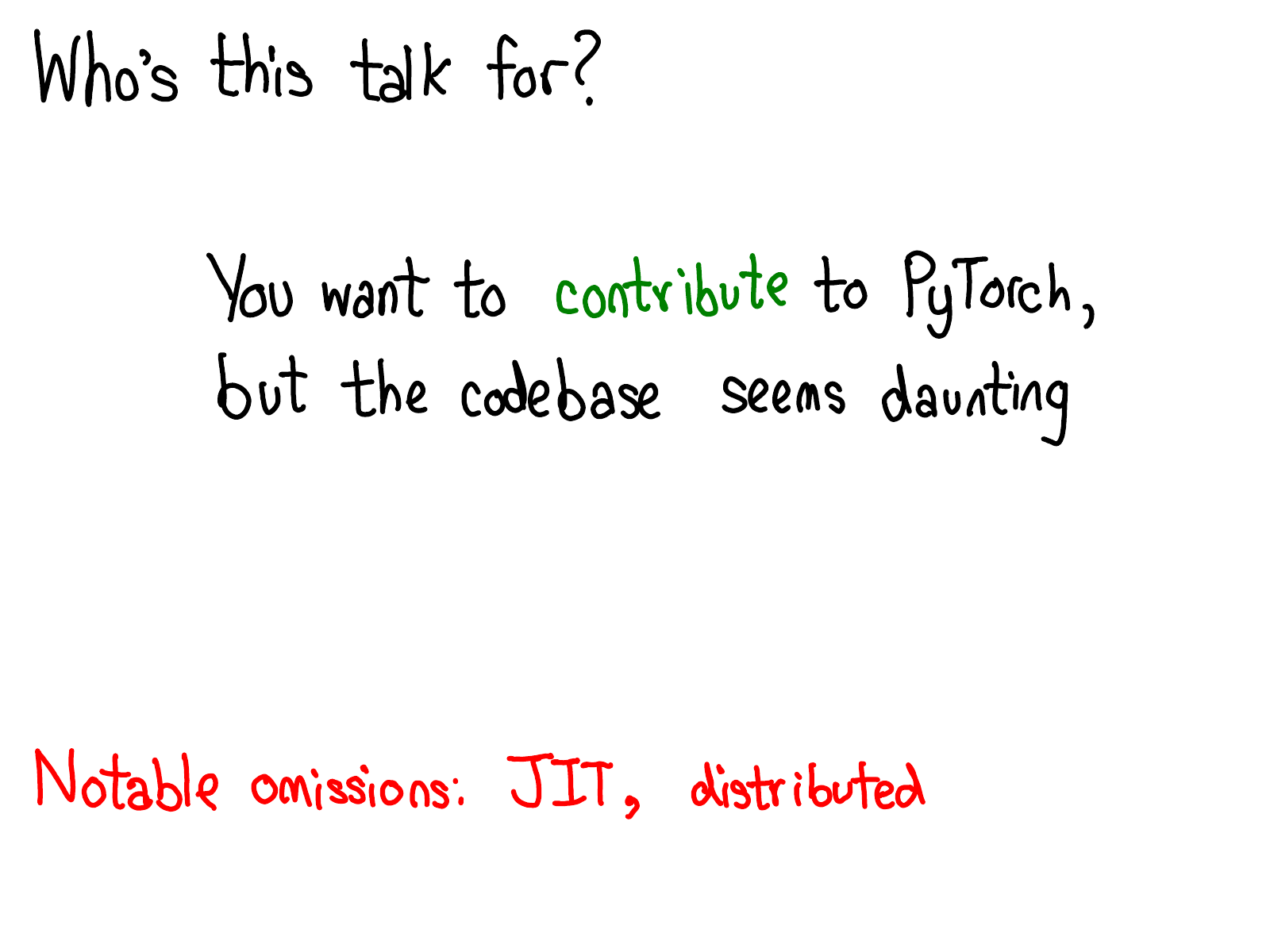
This talk is for those of you who have used PyTorch, and thought to yourself, "It would be great if I could contribute to PyTorch," but were scared by PyTorch's behemoth of a C++ codebase. I'm not going to lie: the PyTorch codebase can be a bit overwhelming at times. The purpose of this talk is to put a map in your hands: to tell you about the basic conceptual structure of a "tensor library that supports automatic differentiation", and give you some tools and tricks for finding your way around the codebase. I'm going to assume that you've written some PyTorch before, but haven't necessarily delved deeper into how a machine learning library is written.

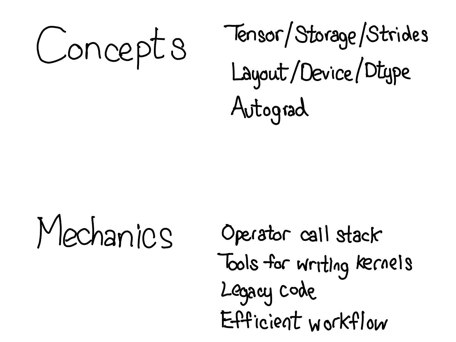
The talk is in two parts: in the first part, I'm going to first introduce you to the conceptual universe of a tensor library. I'll start by talking about the tensor data type you know and love, and give a more detailed discussion about what exactly this data type provides, which will lead us to a better understanding of how it is actually implemented under the hood. If you're an advanced user of PyTorch, you'll be familiar with most of this material. We'll also talk about the trinity of "extension points", layout, device and dtype, which guide how we think about extensions to the tensor class. In the live talk at PyTorch NYC, I skipped the slides about autograd, but I'll talk a little bit about them in these notes as well.

The second part grapples with the actual nitty gritty details involved with actually coding in PyTorch. I'll tell you how to cut your way through swaths of autograd code, what code actually matters and what is legacy, and also all of the cool tools that PyTorch gives you for writing kernels.

---

The tensor is the central data structure in PyTorch. You probably have a pretty good idea about what a tensor intuitively represents: its an n-dimensional data structure containing some sort of scalar type, e.g., floats, ints, et cetera. We can think of a tensor as consisting of some data, and then some metadata describing the size of the tensor, the type of the elements in contains (dtype), what device the tensor lives on (CPU memory? CUDA memory?)

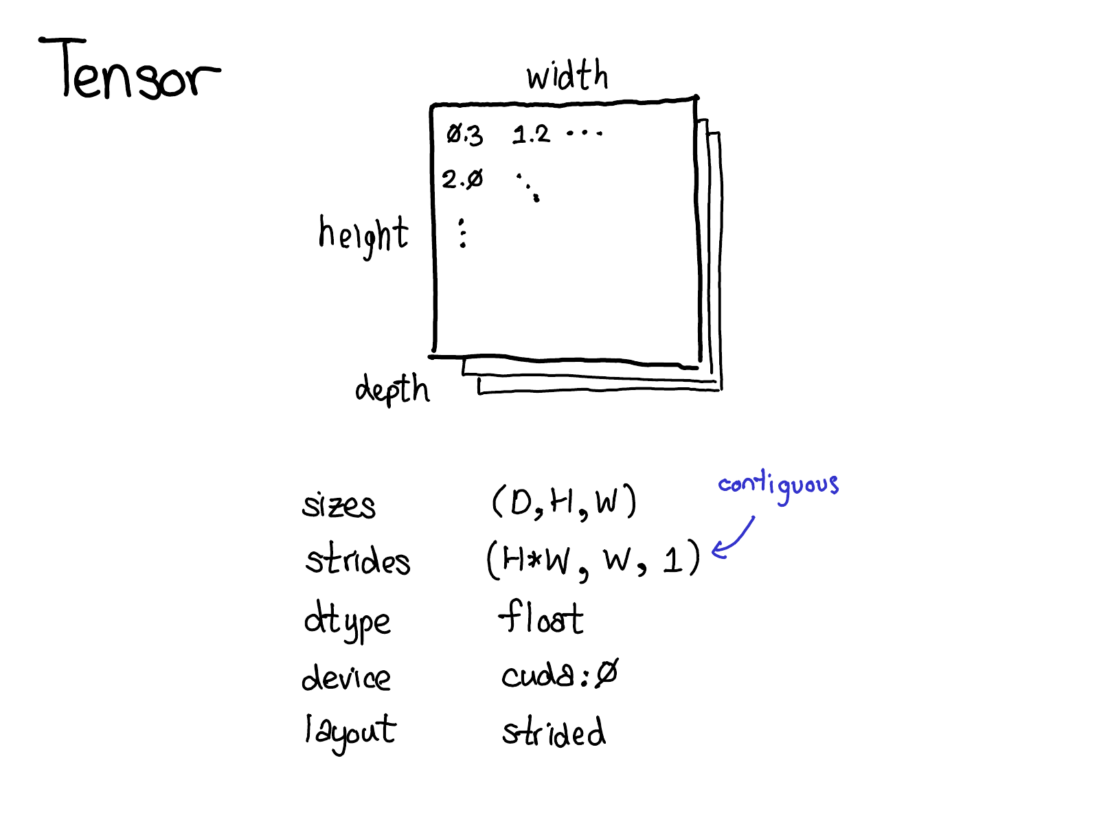
There's also a little piece of metadata you might be less familiar with: the stride. Strides are actually one of the distinctive features of PyTorch, so it's worth discussing them a little more.

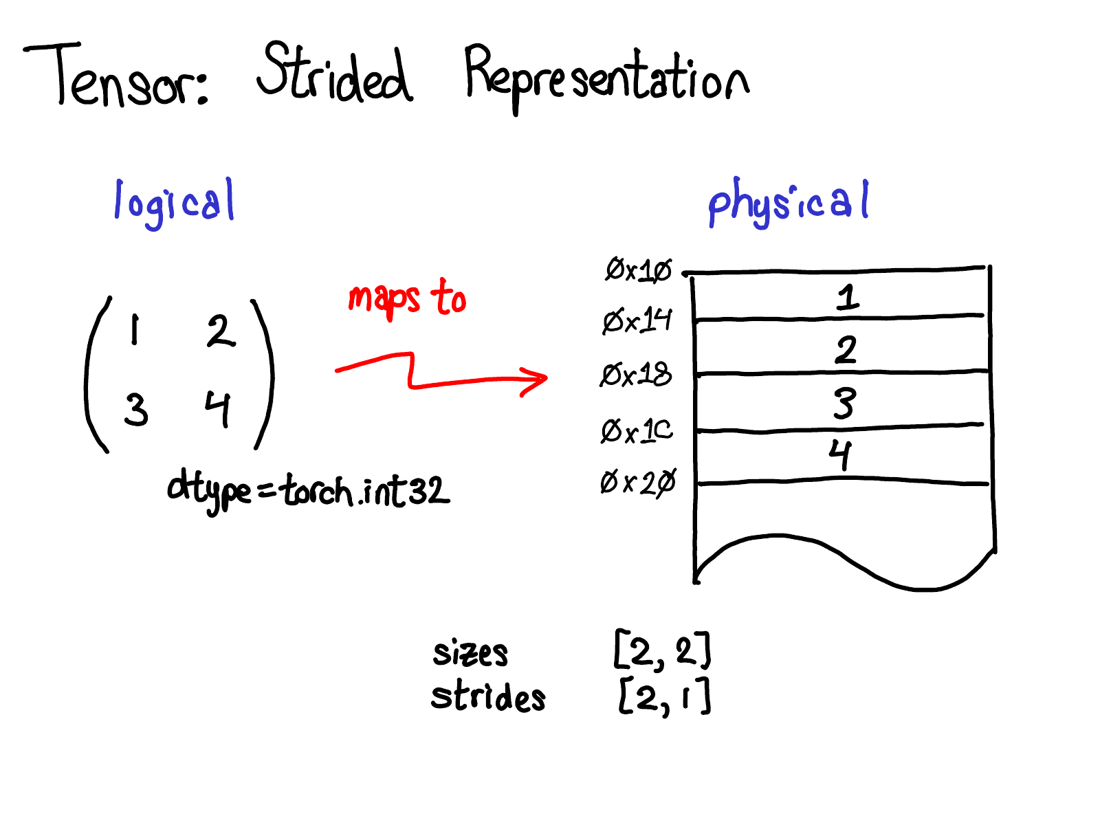
A tensor is a mathematical concept. But to represent it on our computers, we have to define some sort of physical representation for them. The most common representation is to lay out each element of the tensor contiguously in memory (that's where the term contiguous comes from), writing out each row to memory, as you see above. In the example above, I've specified that the tensor contains 32-bit integers, so you can see that each integer lies in a physical address, each offset four bytes from each other. To remember what the actual dimensions of the tensor are, we have to also record what the sizes are as extra metadata.

So, what do strides have to do with this picture?

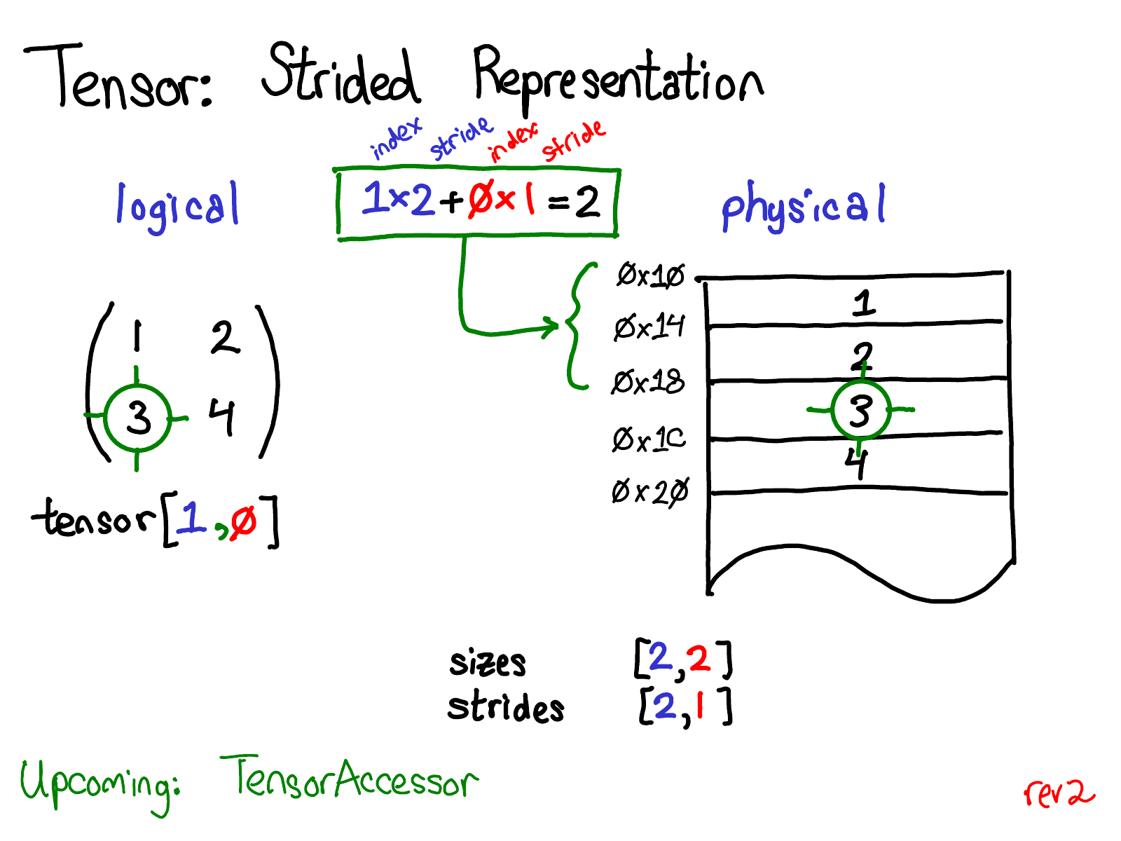
Suppose that I want to access the element at position tensor[1, 0] in my logical representation. How do I translate this logical position into a location in physical memory? Strides tell me how to do this: to find out where any element for a tensor lives, I multiply each index with the respective stride for that dimension, and sum them all together. In the picture above, I've color coded the first dimension blue and the second dimension red, so you can follow the index and stride in the stride calculation. Doing this sum, I get two (zero-indexed), and indeed, the number three lives two below the beginning of the contiguous array.

(Later in the talk, I'll talk about TensorAccessor, a convenience class that handles the indexing calculation. When you use TensorAccessor, rather than raw pointers, this calculation is handled under the covers for you.)

Strides are the fundamental basis of how we provide views to PyTorch users. For example, suppose that I want to extract out a tensor that represents the second row of the tensor above:

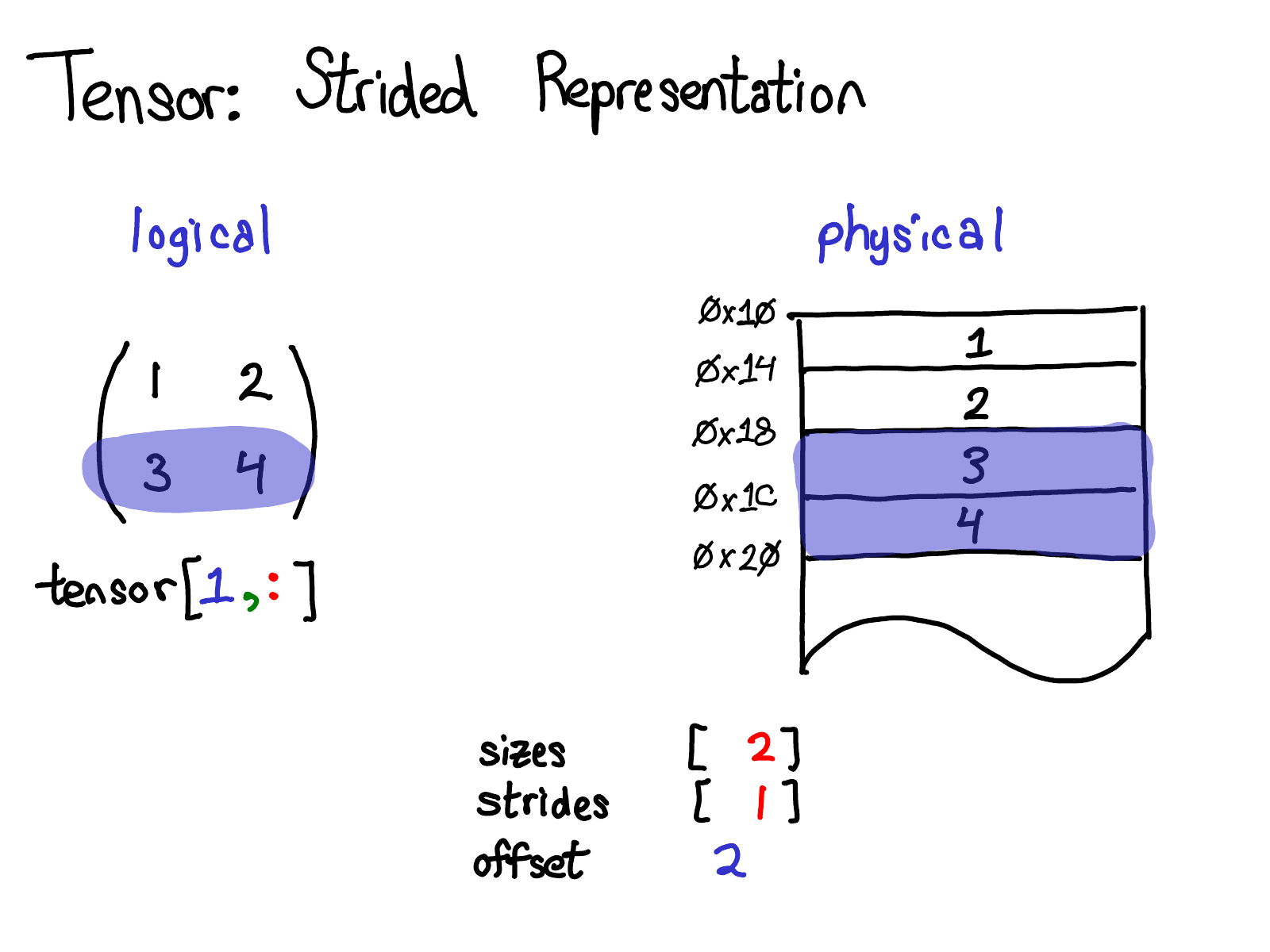
Using advanced indexing support, I can just write tensor[1, :] to get this row. Here's the important thing: when I do this, I don't create a new tensor; instead, I just return a tensor which is a different view on the underlying data. This means that if I, for example, edit the data in that view, it will be reflected in the original tensor. In this case, it's not too hard to see how to do this: three and four live in contiguous memory, and all we need to do is record an offset saying that the data of this (logical) tensor lives two down from the top. (Every tensor records an offset, but most of the time it's zero, and I'll omit it from my diagrams when that's the case.)

Question from the talk: If I take a view on a tensor, how do I free the memory of the underlying tensor?

Answer: You have to make a copy of the view, thus disconnecting it from the original physical memory. There's really not much else you can do. By the way, if you have written Java in the old days, taking substrings of strings has a similar problem, because by default no copy is made, so the substring retains the (possibly very large string). Apparently, they fixed this in Java 7u6.

A more interesting case is if I want to take the first column:

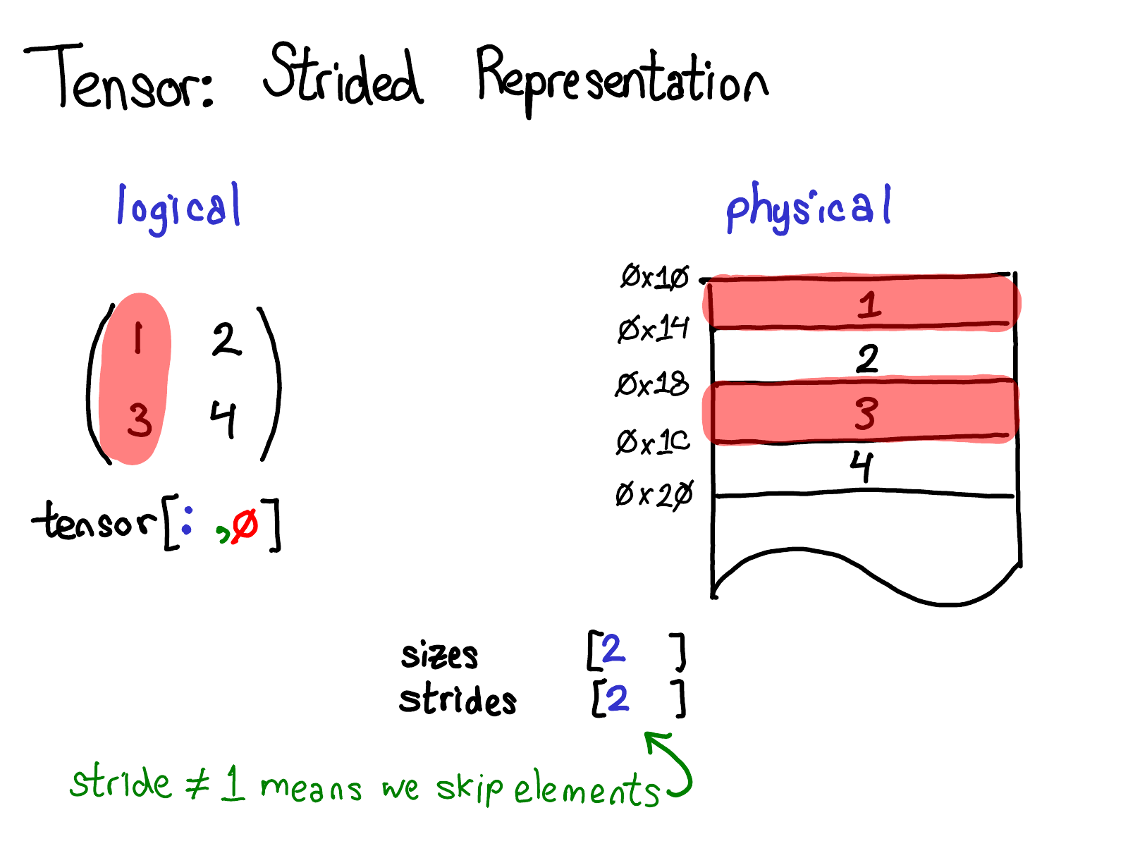
When we look at the physical memory, we see that the elements of the column are not contiguous: there's a gap of one element between each one. Here, strides come to the rescue: instead of specifying a stride of one, we specify a stride of two, saying that between one element and the next, you need to jump two slots. (By the way, this is why it's called a "stride": if we think of an index as walking across the layout, the stride says how many locations we stride forward every time we take a step.)

The stride representation can actually let you represent all sorts of interesting views on tensors; if you want to play around with the possibilities, check out the Stride Visualizer.

Let's step back for a moment, and think about how we would actually implement this functionality (after all, this is an internals talk.) If we can have views on tensor, this means we have to decouple the notion of the tensor (the user-visible concept that you know and love), and the actual physical data that stores the data of the tensor (called storage):

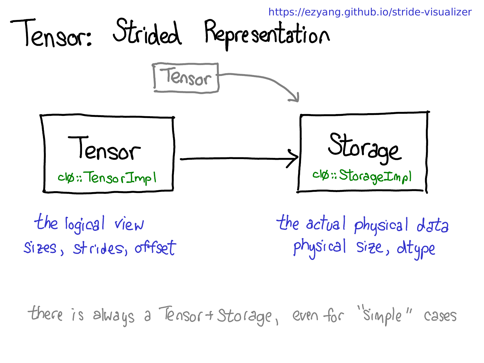
There may be multiple tensors which share the same storage. Storage defines the dtype and physical size of the tensor, while each tensor records the sizes, strides and offset, defining the logical interpretation of the physical memory.

One thing to realize is that there is always a pair of Tensor-Storage, even for "simple" cases where you don't really need a storage (e.g., you just allocated a contiguous tensor with torch.zeros(2, 2)).

By the way, we're interested in making this picture not true; instead of having a separate concept of storage, just define a view to be a tensor that is backed by a base tensor. This is a little more complicated, but it has the benefit that contiguous tensors get a much more direct representation without the Storage indirection. A change like this would make PyTorch's internal representation a bit more like Numpy's.

---

We've talked quite a bit about the data layout of tensor (some might say, if you get the data representation right, everything else falls in place). But it's also worth briefly talking about how operations on the tensor are implemented. At the very most abstract level, when you call torch.mm, two dispatches happen:

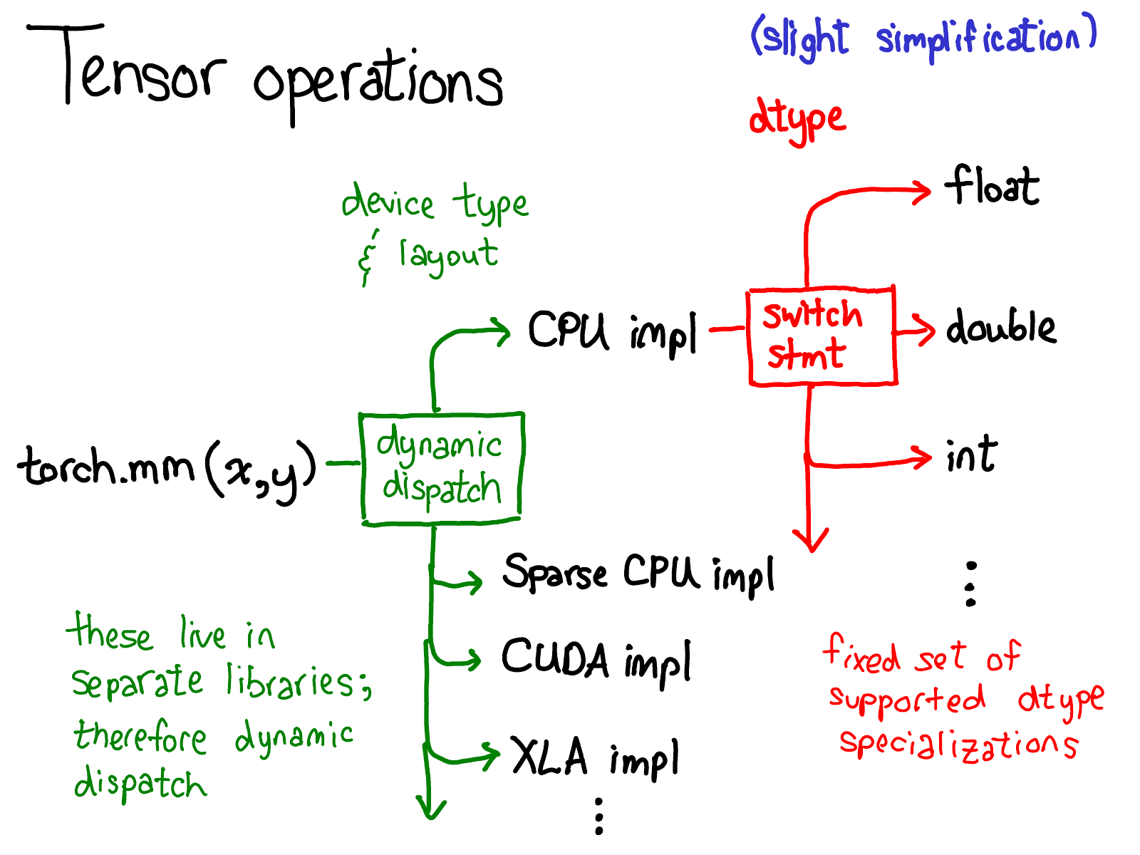
The first dispatch is based on the device type and layout of a tensor: e.g., whether or not it is a CPU tensor or a CUDA tensor (and also, e.g., whether or not it is a strided tensor or a sparse one). This is a dynamic dispatch: it's a virtual function call (exactly where that virtual function call occurs will be the subject of the second half of this talk). It should make sense that you need to do a dispatch here: the implementation of CPU matrix multiply is quite different from a CUDA implementation. It is a dynamic dispatch because these kernels may live in separate libraries (e.g., libcaffe2.so versus libcaffe2_gpu.so), and so you have no choice: if you want to get into a library that you don't have a direct dependency on, you have to dynamic dispatch your way there.

The second dispatch is a dispatch on the dtype in question. This dispatch is just a simple switch-statement for whatever dtypes a kernel chooses to support. Upon reflection, it should also make sense that we need to a dispatch here: the CPU code (or CUDA code, as it may) that implements multiplication on float is different from the code for int. It stands to reason you need separate kernels for each dtype.

This is probably the most important mental picture to have in your head, if you're trying to understand the way operators in PyTorch are invoked. We'll return to this picture when it's time to look more at code.

---

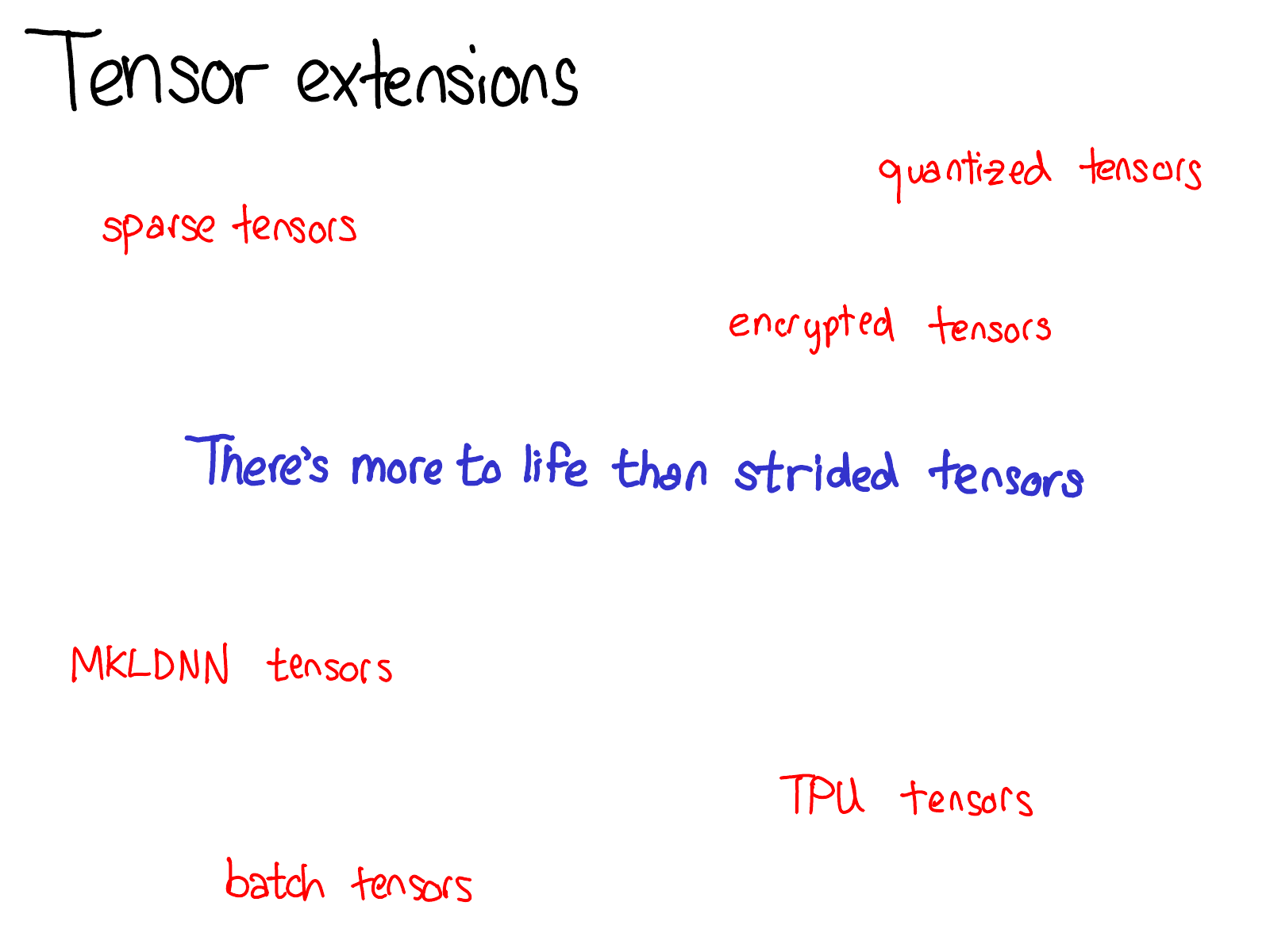
Since we have been talking about Tensor, I also want to take a little time to the world of tensor extensions. After all, there's more to life than dense, CPU float tensors. There's all sorts of interesting extensions going on, like XLA tensors, or quantized tensors, or MKL-DNN tensors, and one of the things we have to think about, as a tensor library, is how to accommodate these extensions.

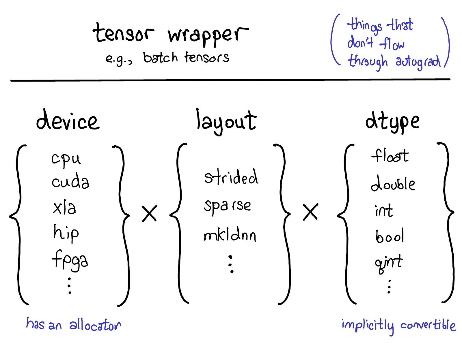
Our current model for extensions offers four extension points on tensors. First, there is the trinity three parameters which uniquely determine what a tensor is:

• The device, the description of where the tensor's physical memory is actually stored, e.g., on a CPU, on an NVIDIA GPU (cuda), or perhaps on an AMD GPU (hip) or a TPU (xla). The distinguishing characteristic of a device is that it has its own allocator, that doesn't work with any other device.
• The layout, which describes how we logically interpret this physical memory. The most common layout is a strided tensor, but sparse tensors have a different layout involving a pair of tensors, one for indices, and one for data; MKL-DNN tensors may have even more exotic layout, like blocked layout, which can't be represented using merely strides.
• The dtype, which describes what it is that is actually stored in each element of the tensor. This could be floats or integers, or it could be, for example, quantized integers.

If you want to add an extension to PyTorch tensors (by the way, if that's what you want to do, please talk to us! None of these things can be done out-of-tree at the moment), you should think about which of these parameters you would extend. The Cartesian product of these parameters define all of the possible tensors you can make. Now, not all of these combinations may actually have kernels (who's got kernels for sparse, quantized tensors on FPGA?) but in principle the combination could make sense, and thus we support expressing it, at the very least.

There's one last way you can make an "extension" to Tensor functionality, and that's write a wrapper class around PyTorch tensors that implements your object type. This perhaps sounds obvious, but sometimes people reach for extending one of the three parameters when they should have just made a wrapper class instead. One notable merit of wrapper classes is they can be developed entirely out of tree.

When should you write a tensor wrapper, versus extending PyTorch itself? The key test is whether or not you need to pass this tensor along during the autograd backwards pass. This test, for example, tells us that sparse tensor should be a true tensor extension, and not just a Python object that contains an indices and values tensor: when doing optimization on networks involving embeddings, we want the gradient generated by the embedding to be sparse.

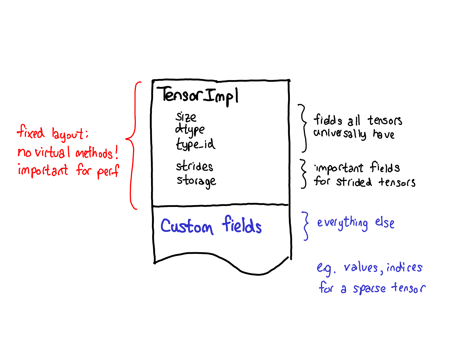
Our philosophy on extensions also has an impact of the data layout of tensor itself. One thing we really want out of our tensor struct is for it to have a fixed layout: we don't want fundamental (and very frequently called) operations like "What's the size of a tensor?" to require virtual dispatches. So when you look at the actual layout of a Tensor (defined in the TensorImpl struct), what we see is a common prefix of all fields that we consider all "tensor"-like things to universally have, plus a few fields that are only really applicable for strided tensors, but are so important that we've kept them in the main struct, and then a suffix of custom fields that can be done on a per-Tensor basis. Sparse tensors, for example, store their indices and values in this suffix.

---

I told you all about tensors, but if that was the only thing PyTorch provided, we'd basically just be a Numpy clone. The distinguishing characteristic of PyTorch when it was originally released was that it provided automatic differentiation on tensors (these days, we have other cool features like TorchScript; but back then, this was it!)

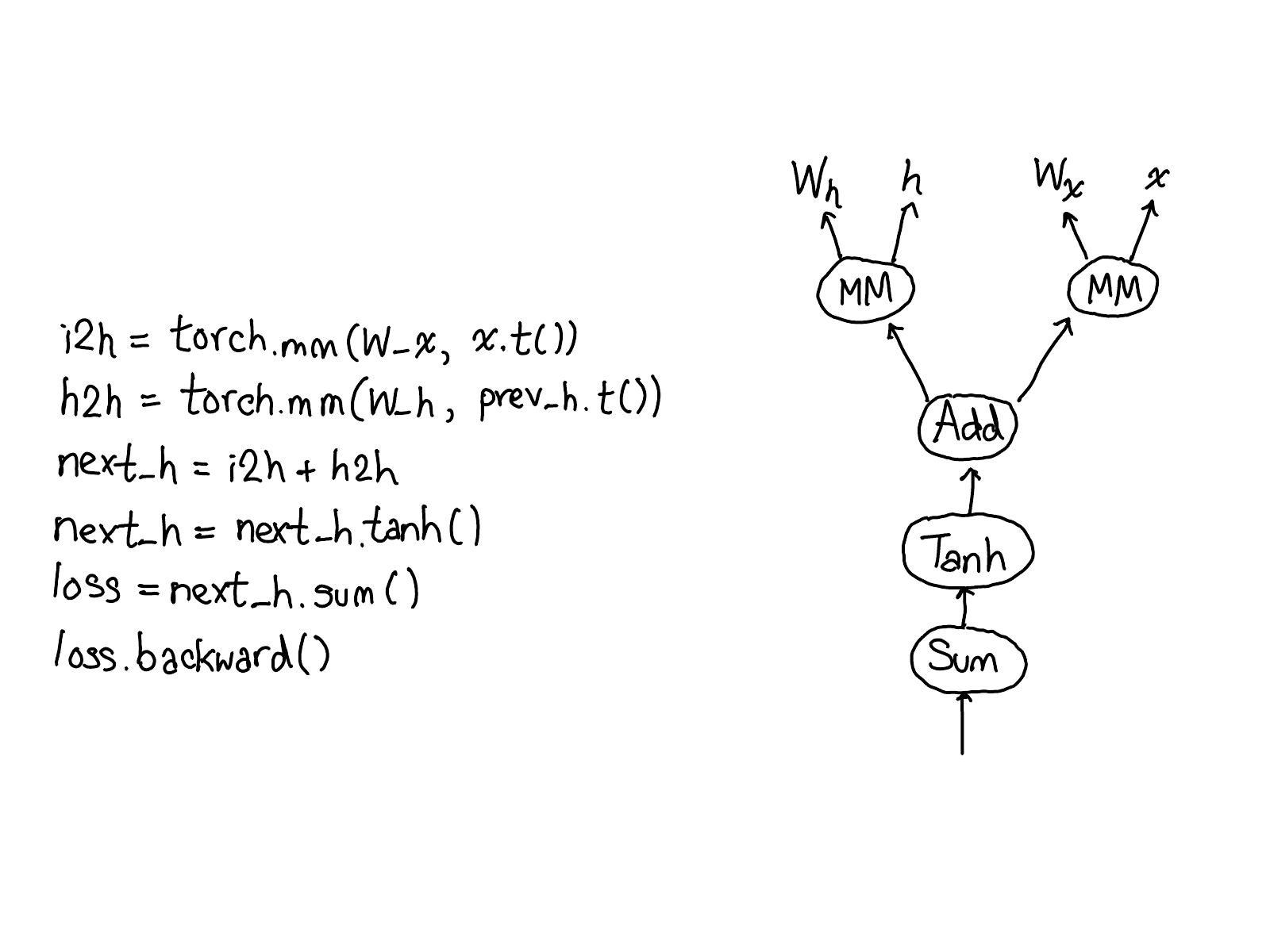
What does automatic differentiation do? It's the machinery that's responsible for taking a neural network:

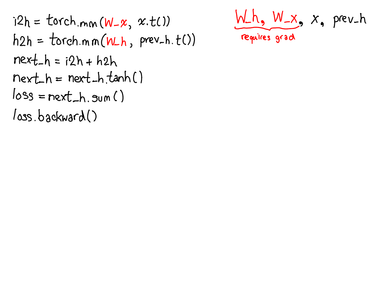
...and fill in the missing code that actually computes the gradients of your network:

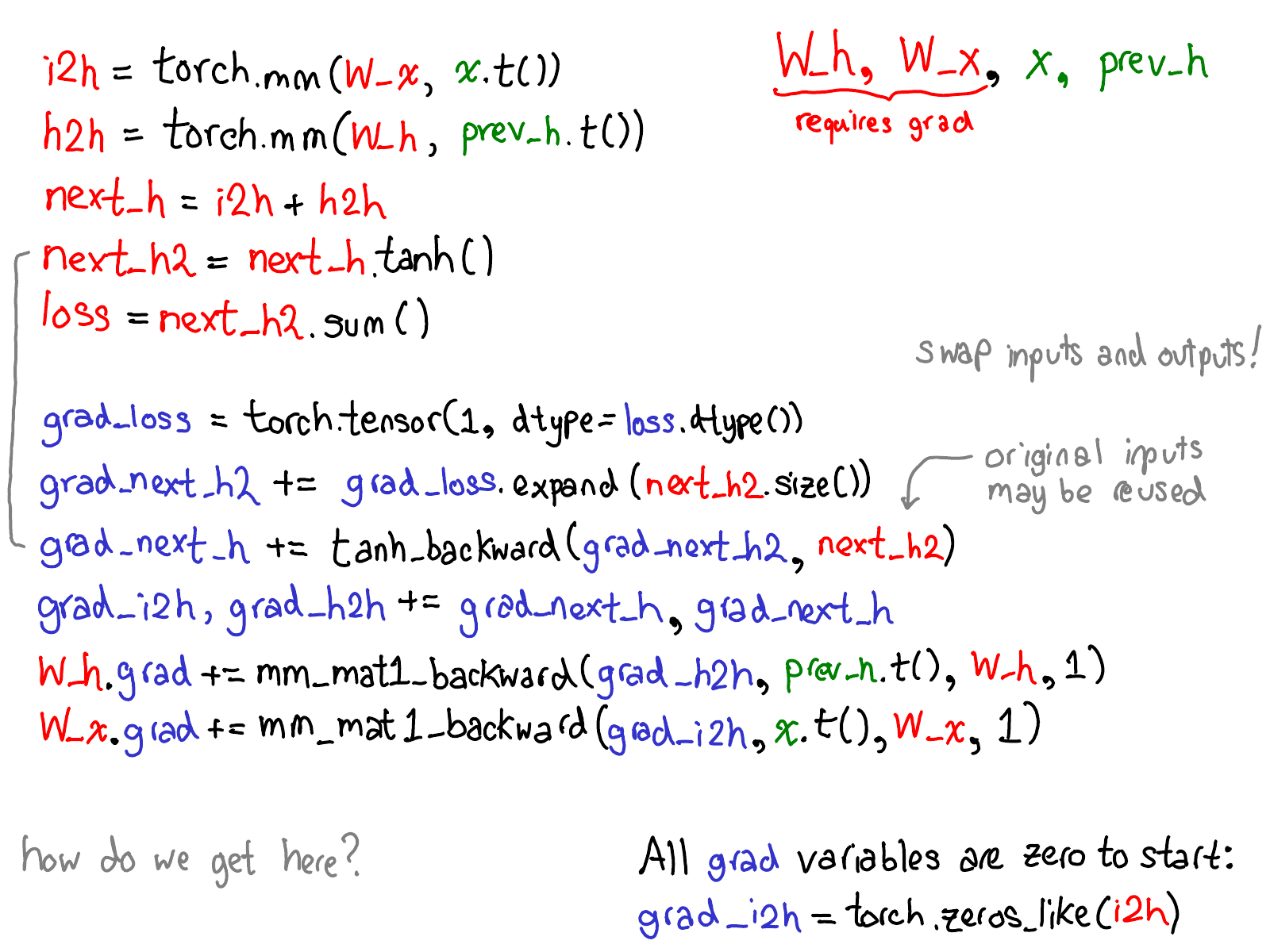
Take a moment to study this diagram. There's a lot to unpack; here's what to look at:

1. First, rest your eyes on the variables in red and blue. PyTorch implements reverse-mode automatic differentiation, which means that we effectively walk the forward computations "backward" to compute the gradients. You can see this if you look at the variable names: at the bottom of the red, we compute loss; then, the first thing we do in the blue part of the program is compute grad_loss. loss was computed from next_h2, so we compute grad_next_h2. Technically, these variables which we call grad_ are not really gradients; they're really Jacobians left-multiplied by a vector, but in PyTorch we just call them grad and mostly everyone knows what we mean.
2. If the structure of the code stays the same, the behavior doesn't: each line from forwards is replaced with a different computation, that represents the derivative of the forward operation. For example, the tanh operation is translated into a tanh_backward operation (these two lines are connected via a grey line on the left hand side of the diagram). The inputs and outputs of the forward and backward operations are swapped: if the forward operation produced next_h2, the backward operation takes grad_next_h2 as an input.

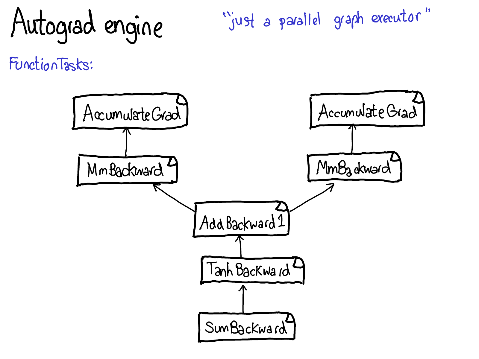
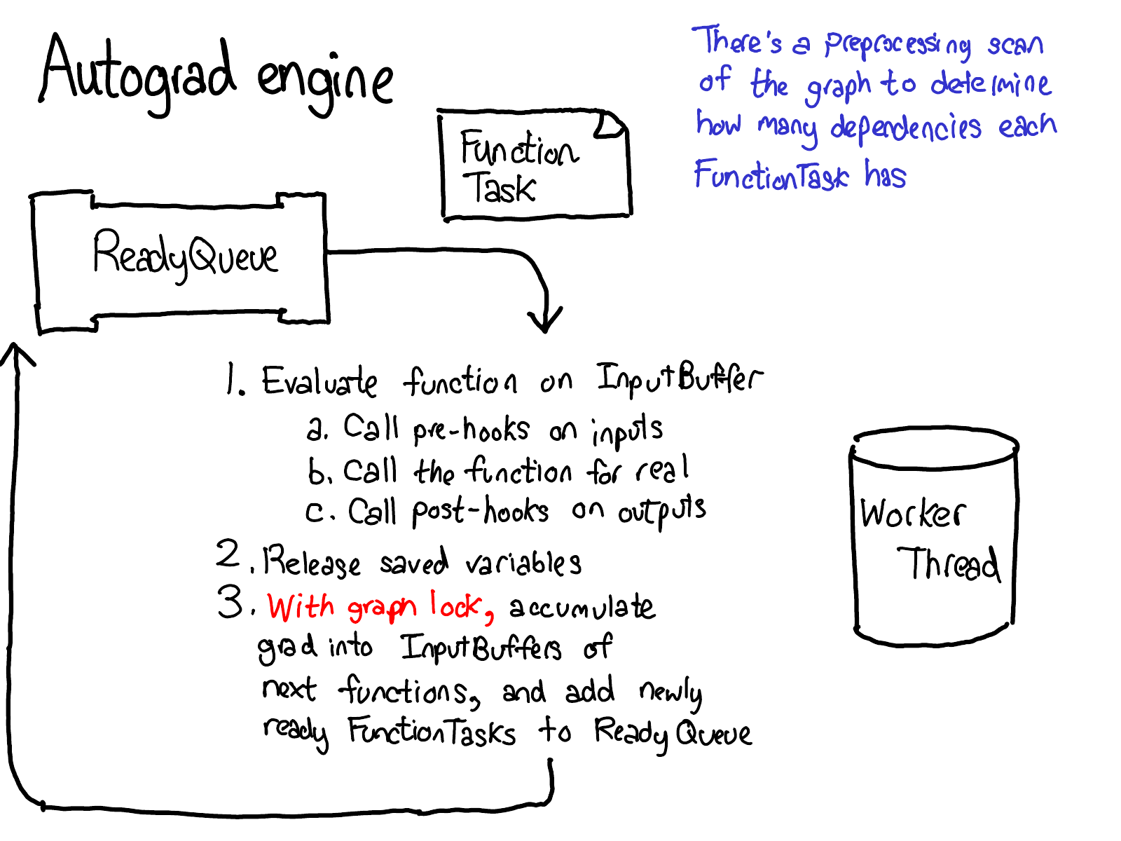
The whole point of autograd is to do the computation that is described by this diagram, but without actually ever generating this source. PyTorch autograd doesn't do a source-to-source transformation (though PyTorch JIT does know how to do symbolic differentiation).

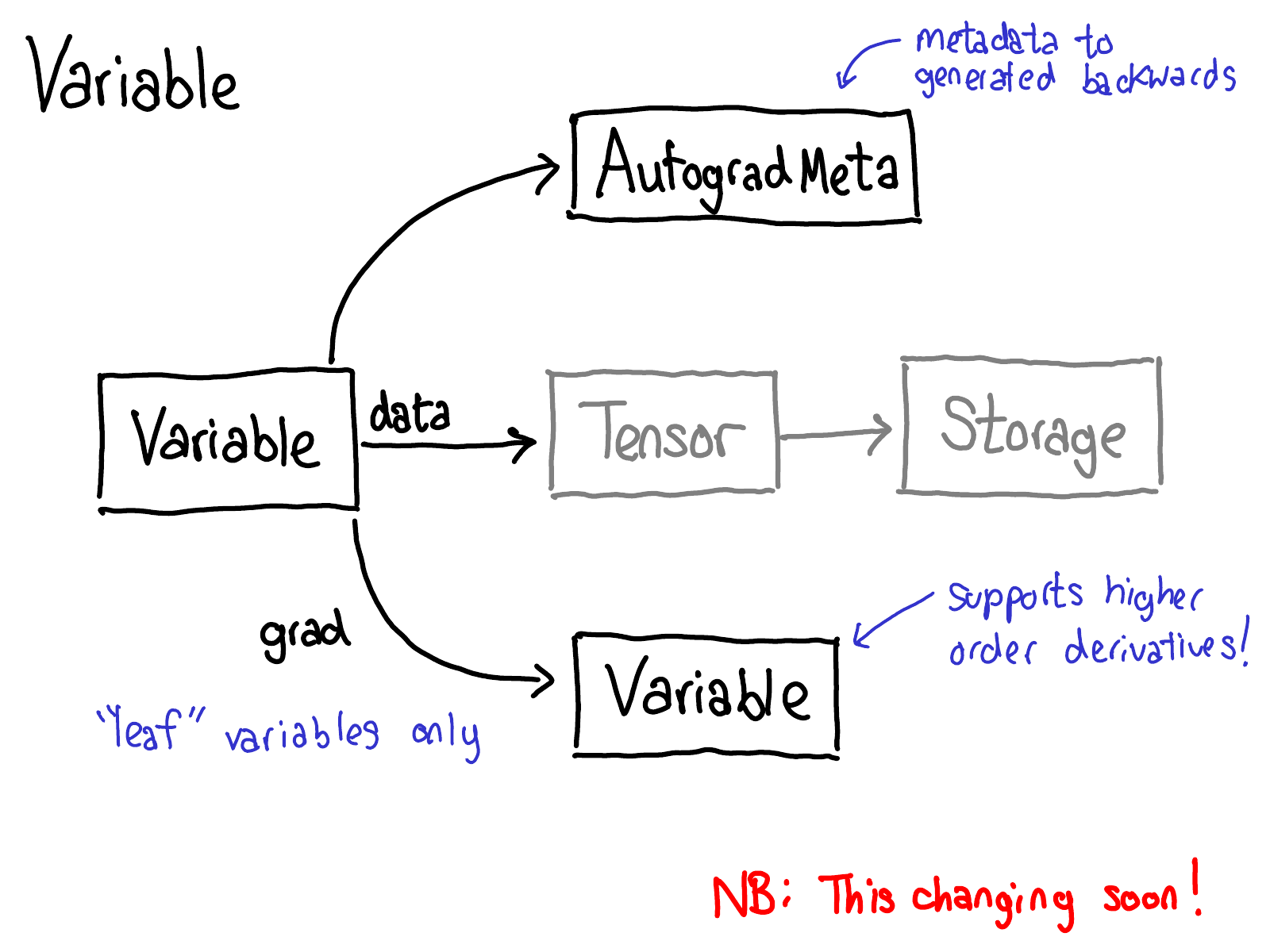
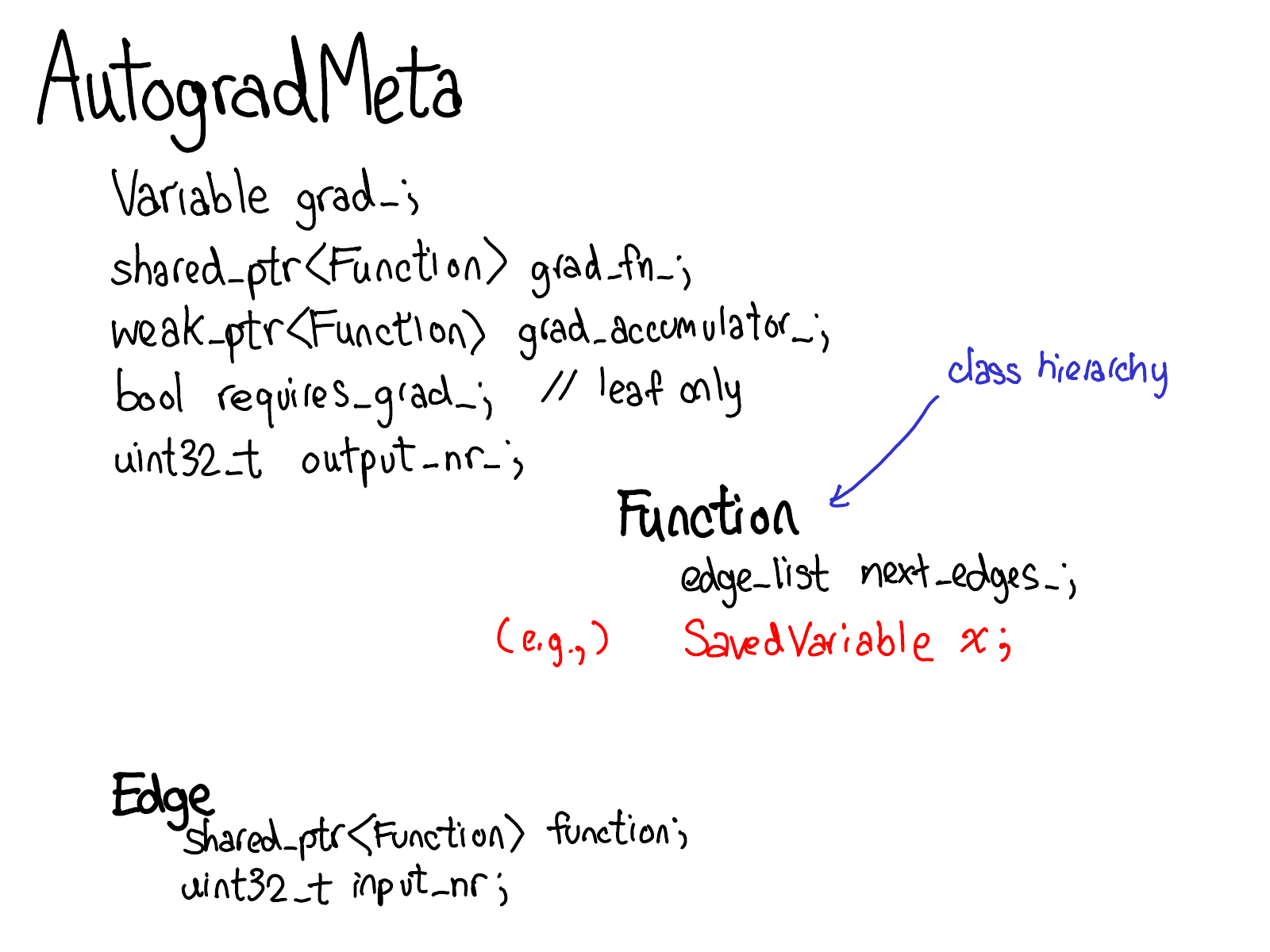
To do this, we need to store more metadata when we carry out operations on tensors. Let's adjust our picture of the tensor data structure: now instead of just a tensor which points to a storage, we now have a variable which wraps this tensor, and also stores more information (AutogradMeta), which is needed for performing autograd when a user calls loss.backward() in their PyTorch script.

This is yet another slide which will hopefully be out of date in the near future. Will Feng is working on a Variable-Tensor merge in C++, following a simple merge which happened to PyTorch's frontend interface.

We also have to update our picture about dispatch:

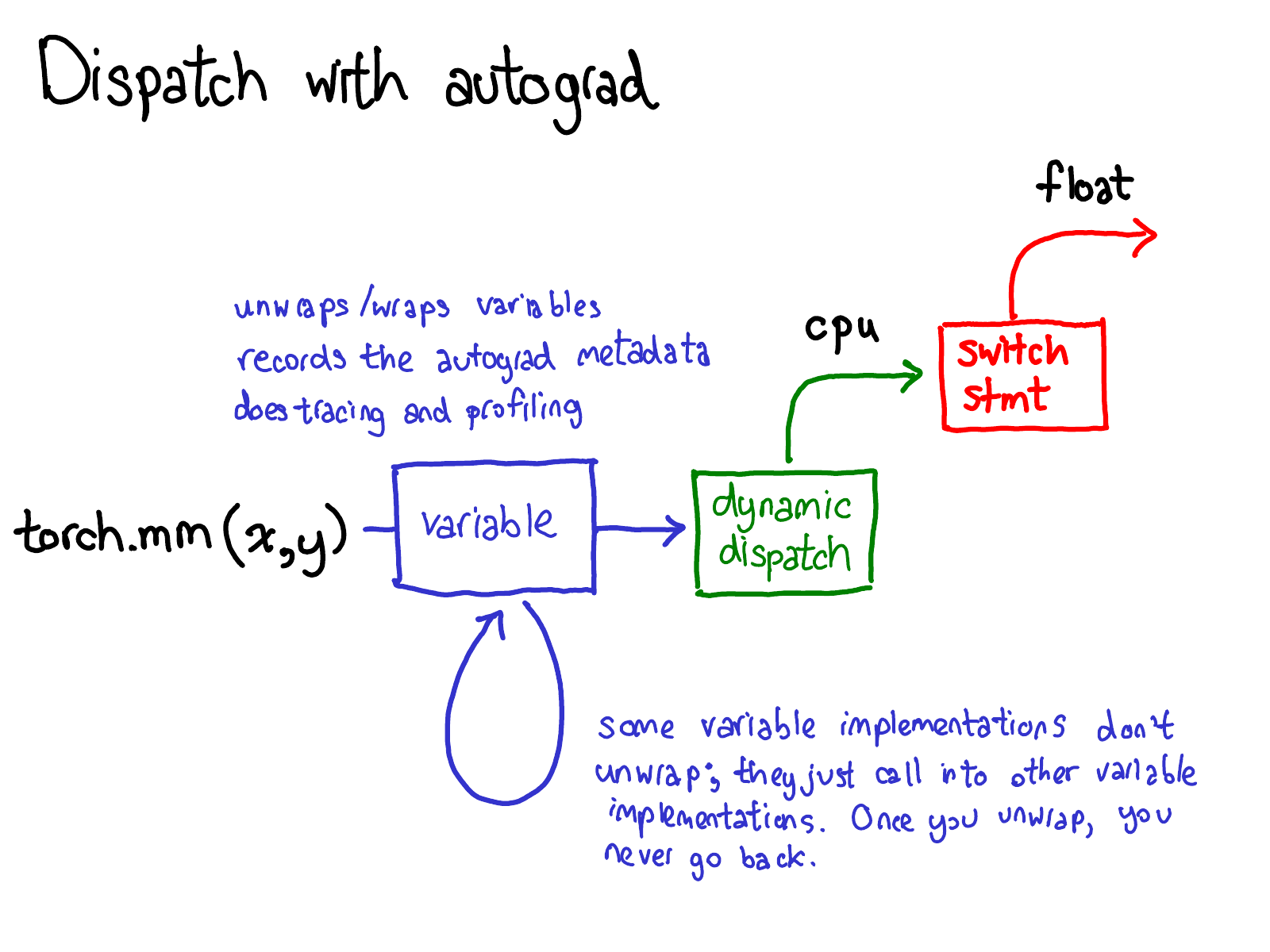
Before we dispatch to CPU or CUDA implementations, there is another dispatch on variables, which is responsible for unwrapping variables, calling the underlying implementation (in green), and then rewrapping the results into variables and recording the necessary autograd metadata for backwards.

Some implementations don't unwrap; they just call into other variable implementations. So you might spend a while in the Variable universe. However, once you unwrap and go into the non-Variable Tensor universe, that's it; you never go back to Variable (except by returning from your function.)

---

In my NY meetup talk, I skipped the following seven slides. I'm also going to delay writeup for them; you'll have to wait for the sequel for some text.

---

Enough about concepts, let's look at some code.

PyTorch has a lot of folders, and there is a very detailed description of what they are in the CONTRIBUTING document, but really, there are only four directories you really need to know about:

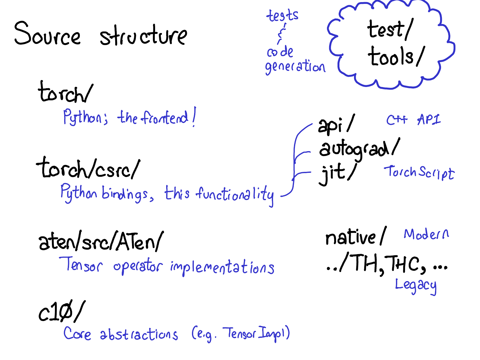
• First, torch/ contains what you are most familiar with: the actual Python modules that you import and use. This stuff is Python code and easy to hack on (just make a change and see what happens). However, lurking not too deep below the surface is...
• torch/csrc/, the C++ code that implements what you might call the frontend of PyTorch. In more descriptive terms, it implements the binding code that translates between the Python and C++ universe, and also some pretty important pieces of PyTorch, like the autograd engine and the JIT compiler. It also contains the C++ frontend code.
• aten/, short for "A Tensor Library" (coined by Zachary DeVito), is a C++ library that implements the operations of Tensors. If you're looking for where some kernel code lives, chances are it's in ATen. ATen itself bifurcates into two neighborhoods of operators: the "native" operators, which are modern, C++ implementations of operators, and the "legacy" operators (TH, THC, THNN, THCUNN), which are legacy, C implementations. The legacy operators are the bad part of town; try not to spend too much time there if you can.
• c10/, which is a pun on Caffe2 and A"Ten" (get it? Caffe 10) contains the core abstractions of PyTorch, including the actual implementations of the Tensor and Storage data structures.

That's a lot of places to look for code; we should probably simplify the directory structure, but that's how it is. If you're trying to work on operators, you'll spend most of your time in aten.

Let's see how this separation of code breaks down in practice:

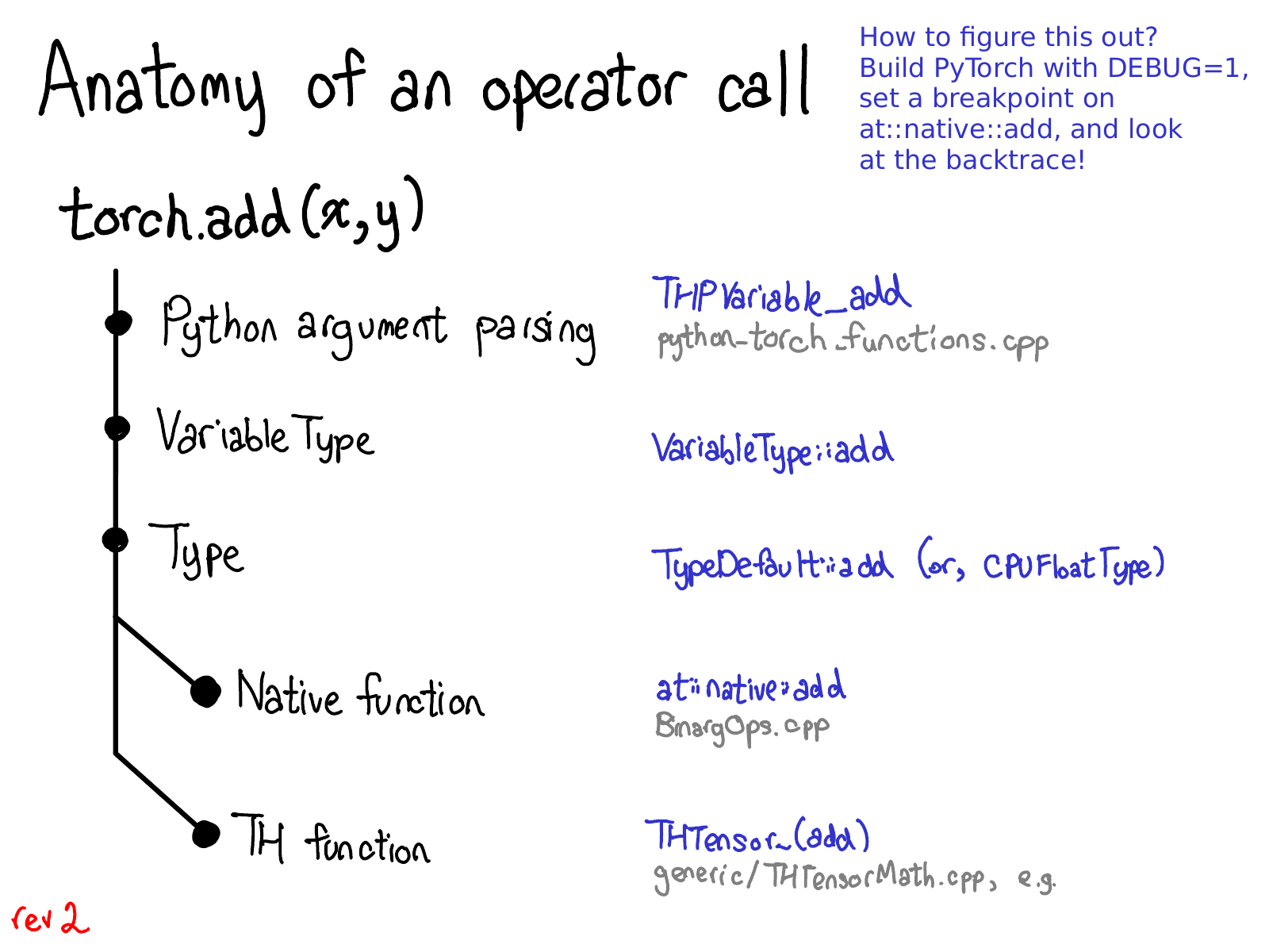
When you call a function like torch.add, what actually happens? If you remember the discussion we had about dispatching, you already have the basic picture in your head:

1. We have to translate from Python realm to the C++ realm (Python argument parsing)
2. We handle variable dispatch (VariableType--Type, by the way, doesn't really have anything to do programming language types, and is just a gadget for doing dispatch.)
3. We handle device type / layout dispatch (Type)
4. We have the actual kernel, which is either a modern native function, or a legacy TH function.

Each of these steps corresponds concretely to some code. Let's cut our way through the jungle.

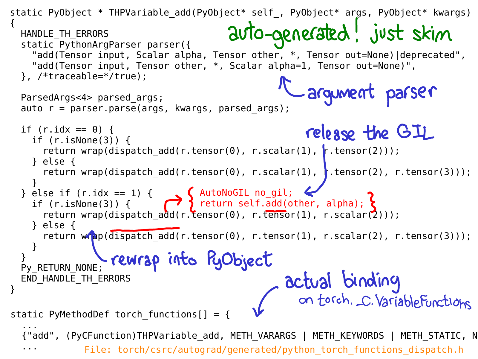
Our initial landing point in the C++ code is the C implementation of a Python function, which we've exposed to the Python side as something like torch._C.VariableFunctions.add. THPVariable_add is the implementation of one such implementation.

One important thing to know about this code is that it is auto-generated. If you search in the GitHub repository, you won't find it, because you have to actually build PyTorch to see it. Another important thing is, you don't have to really deeply understand what this code is doing; the idea is to skim over it and get a sense for what it is doing. Above, I've annotated some of the most important bits in blue: you can see that there is a use of a class PythonArgParser to actually pull out C++ objects out of the Python args and kwargs; we then call a dispatch_add function (which I've inlined in red); this releases the global interpreter lock and then calls a plain old method on the C++ Tensor self. On its way back, we rewrap the returned Tensor back into a PyObject.

(At this point, there's an error in the slides: I'm supposed to tell you about the Variable dispatch code. I haven't fixed it here yet. Some magic happens, then...)

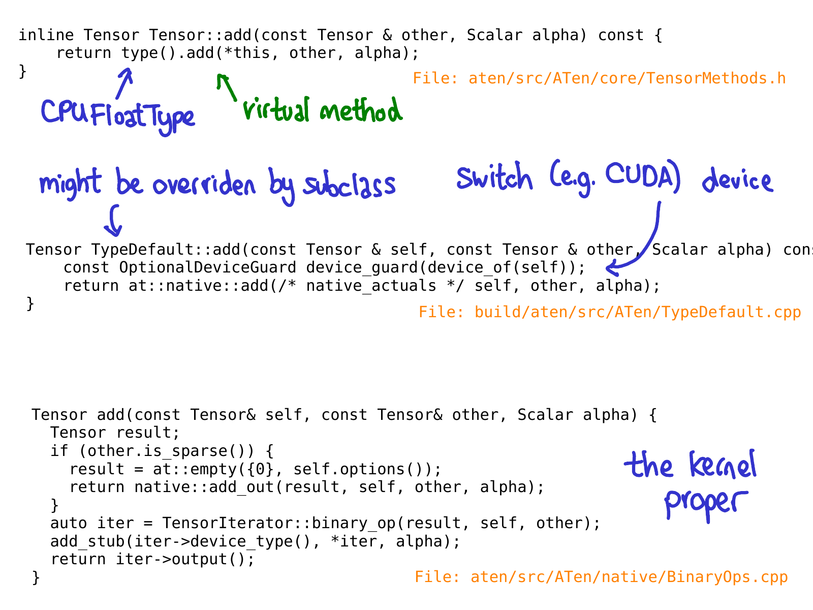
When we call the add method on the Tensor class, no virtual dispatch happens yet. Instead, we have an inline method which calls a virtual method on a "Type" object. This method is the actual virtual method (this is why I say Type is just a "gadget" that gets you dynamic dispatch.) In the particular case of this example, this virtual call dispatches to an implementation of add on a class named TypeDefault. This happens to be because we have an implementation of add that is the same for every device type (both CPU and CUDA); if we had happened to have different implementations, we might have instead landed on something like CPUFloatType::add. It is this implementation of the virtual method that finally gets us to the actual kernel code.

Hopefully, this slide will be out-of-date very soon too; Roy Li is working on replacing Type dispatch with another mechanism which will help us better support PyTorch on mobile.

It's worth reemphasizing that all of the code, until we got to the kernel, is automatically generated.

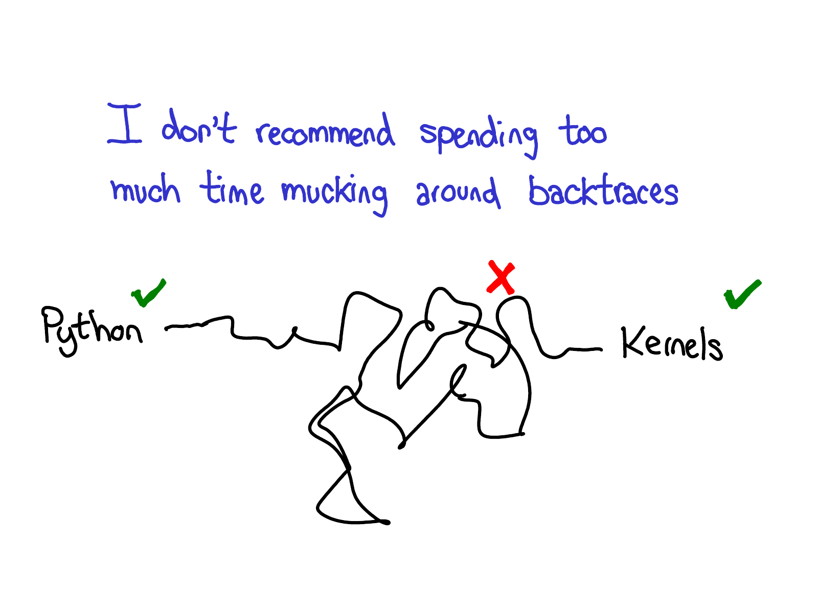
It's a bit twisty and turny, so once you have some basic orientation about what's going on, I recommend just jumping straight to the kernels.

---

PyTorch offers a lot of useful tools for prospective kernel writers. In this section, we'll walk through a few of them. But first of all, what do you need to write a kernel?

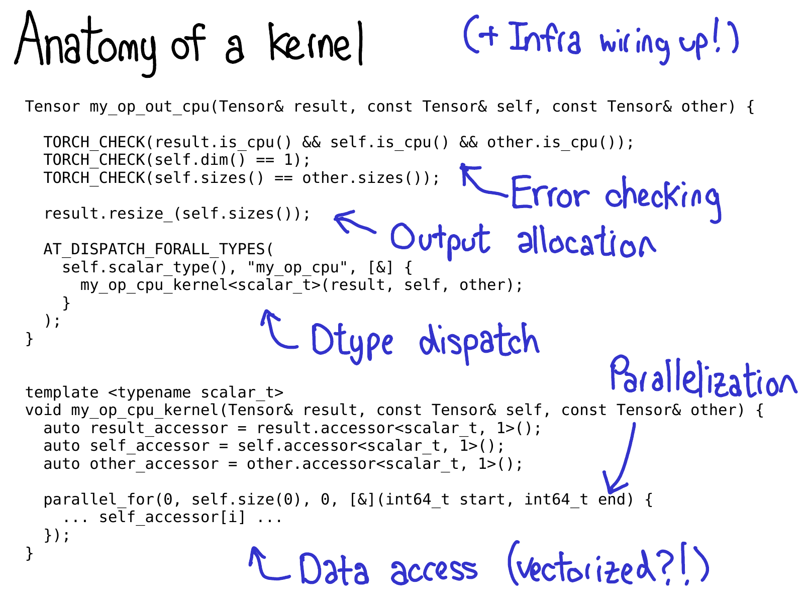
We generally think of a kernel in PyTorch consisting of the following parts:

1. First, there's some metadata which we write about the kernel, which powers the code generation and lets you get all the bindings to Python, without having to write a single line of code.
2. Once you've gotten to the kernel, you're past the device type / layout dispatch. The first thing you need to write is error checking, to make sure the input tensors are the correct dimensions. (Error checking is really important! Don't skimp on it!)
3. Next, we generally have to allocate the result tensor which we are going to write the output into.
4. Time for the kernel proper. At this point, you now should do the second, dtype dispatch, to jump into a kernel which is specialized per dtype it operates on. (You don't want to do this too early, because then you will be uselessly duplicating code that looks the same in any case.)
5. Most performant kernels need some sort of parallelization, so that you can take advantage of multi-CPU systems. (CUDA kernels are "implicitly" parallelized, since their programming model is built on top of massive parallelization).
6. Finally, you need to access the data and do the computation you wanted to do!

In the subsequent slides, we'll walk through some of the tools PyTorch has for helping you implementing these steps.

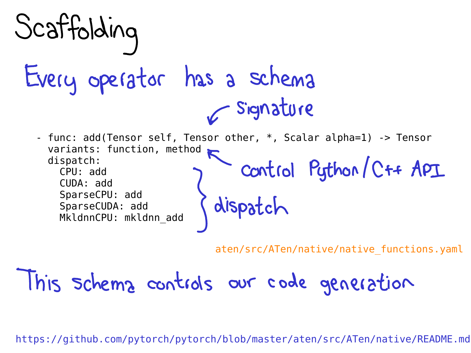
To take advantage of all of the code generation which PyTorch brings, you need to write a schema for your operator. The schema gives a mypy-esque type of your function, and also controls whether or not we generate bindings for methods or functions on Tensor. You also tell the schema what implementations of your operator should be called for given device-layout combinations. Check out the README in native is for more information about this format.

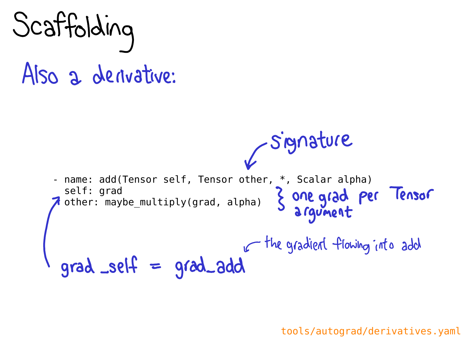
You also may need to define a derivative for your operation in derivatives.yaml.

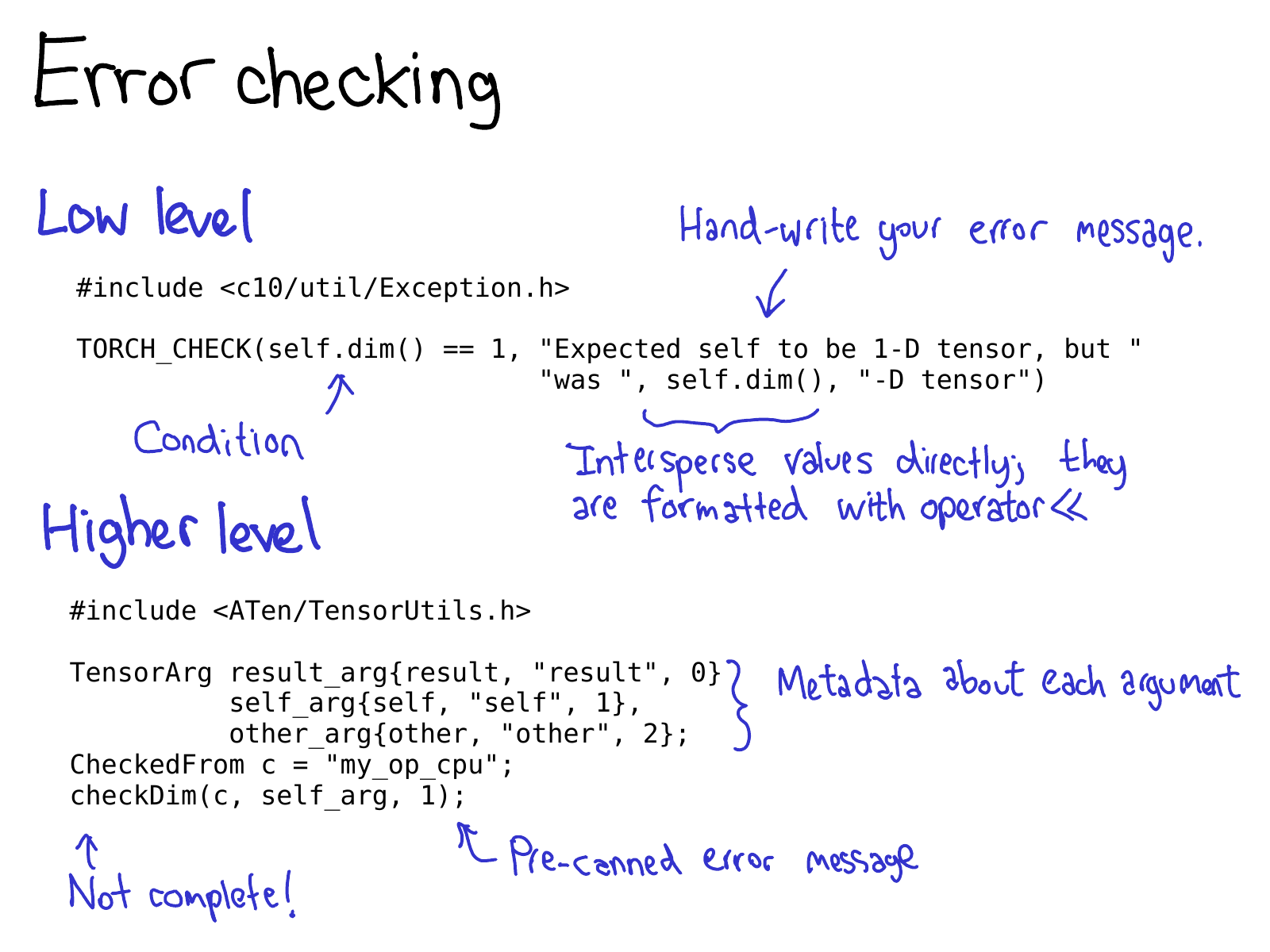
Error checking can be done by way of either a low level or a high level API. The low level API is just a macro, TORCH_CHECK, which takes a boolean, and then any number of arguments to make up the error string to render if the boolean is not true. One nice thing about this macro is that you can intermix strings with non-string data; everything is formatted using their implementation of operator<<, and most important data types in PyTorch have operator<< implementations.

The high level API saves you from having to write up repetitive error messages over and over again. The way it works is you first wrap each Tensor into a TensorArg, which contains information about where the tensor came from (e.g., its argument name). It then provides a number of pre-canned functions for checking various properties; e.g., checkDim() tests if the tensor's dimensionality is a fixed number. If it's not, the function provides a user-friendly error message based on the TensorArg metadata.

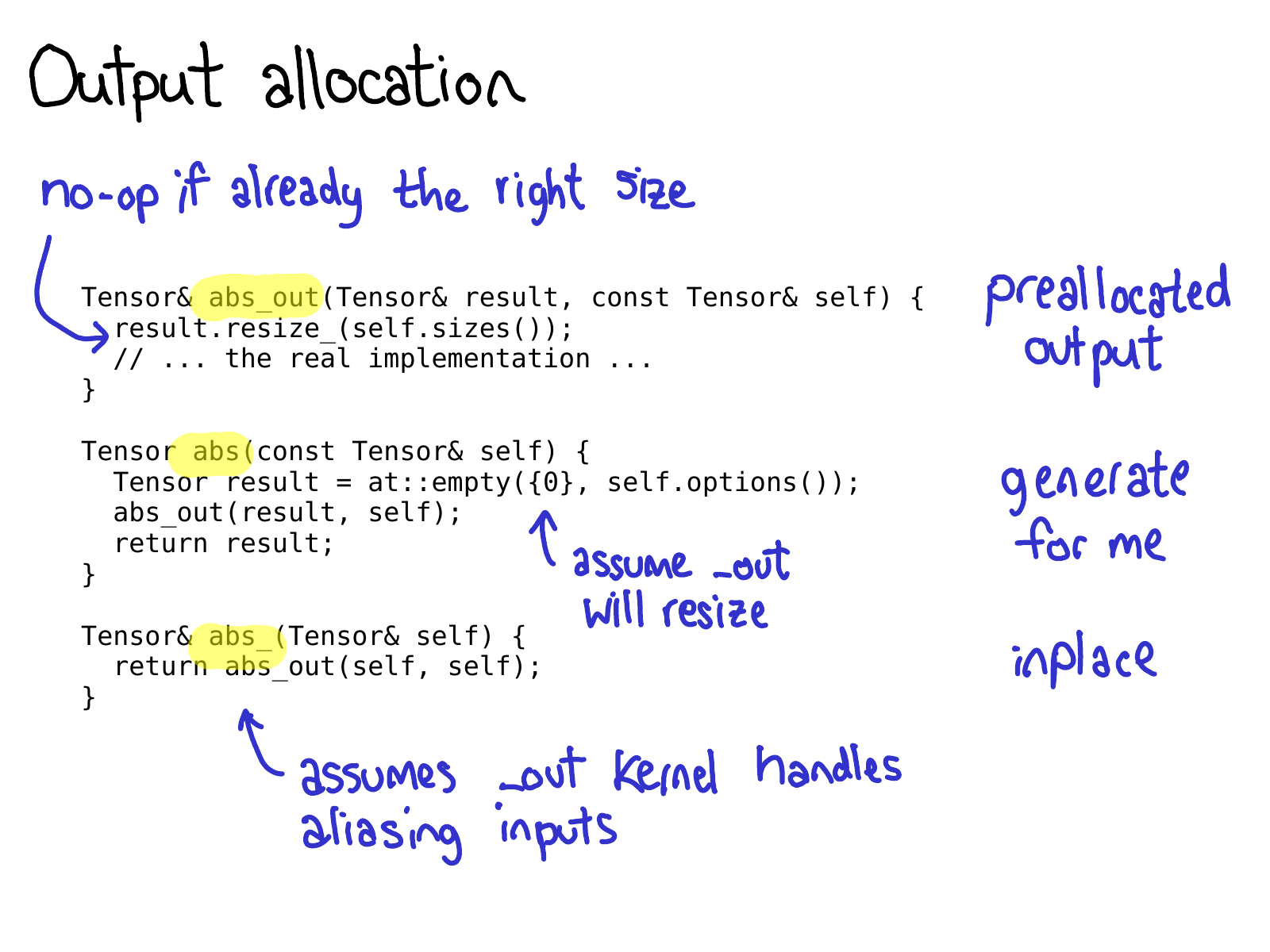
One important thing to be aware about when writing operators in PyTorch, is that you are often signing up to write three operators: abs_out, which operates on a preallocated output (this implements the out= keyword argument), abs_, which operates inplace, and abs, which is the plain old functional version of an operator.

Most of the time, abs_out is the real workhorse, and abs and abs_ are just thin wrappers around abs_out; but sometimes writing specialized implementations for each case are warranted.

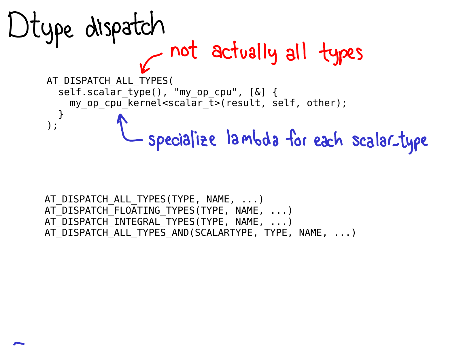
To do dtype dispatch, you should use the AT_DISPATCH_ALL_TYPES macro. This takes in the dtype of the tensor you want to dispatch over, and a lambda which will be specialized for each dtype that is dispatchable from the macro. Usually, this lambda just calls a templated helper function.

This macro doesn't just "do dispatch", it also decides what dtypes your kernel will support. As such, there are actually quite a few versions of this macro, which let you pick different subsets of dtypes to generate specializations for. Most of the time, you'll just want AT_DISPATCH_ALL_TYPES, but keep an eye out for situations when you might want to dispatch to some more types. There's guidance in Dispatch.h for how to select the correct one for your use-case.

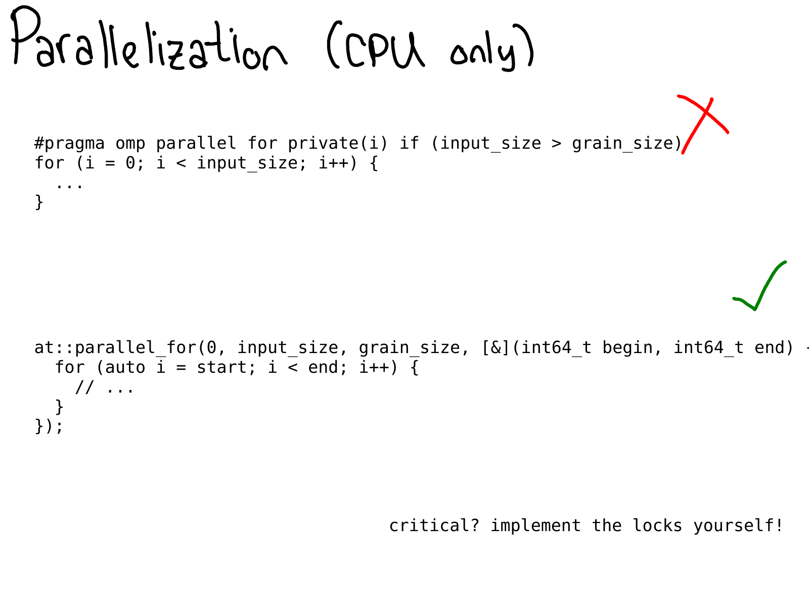
On CPU, you frequently want to parallelize your code. In the past, this was usually done by directly sprinkling OpenMP pragmas in your code.

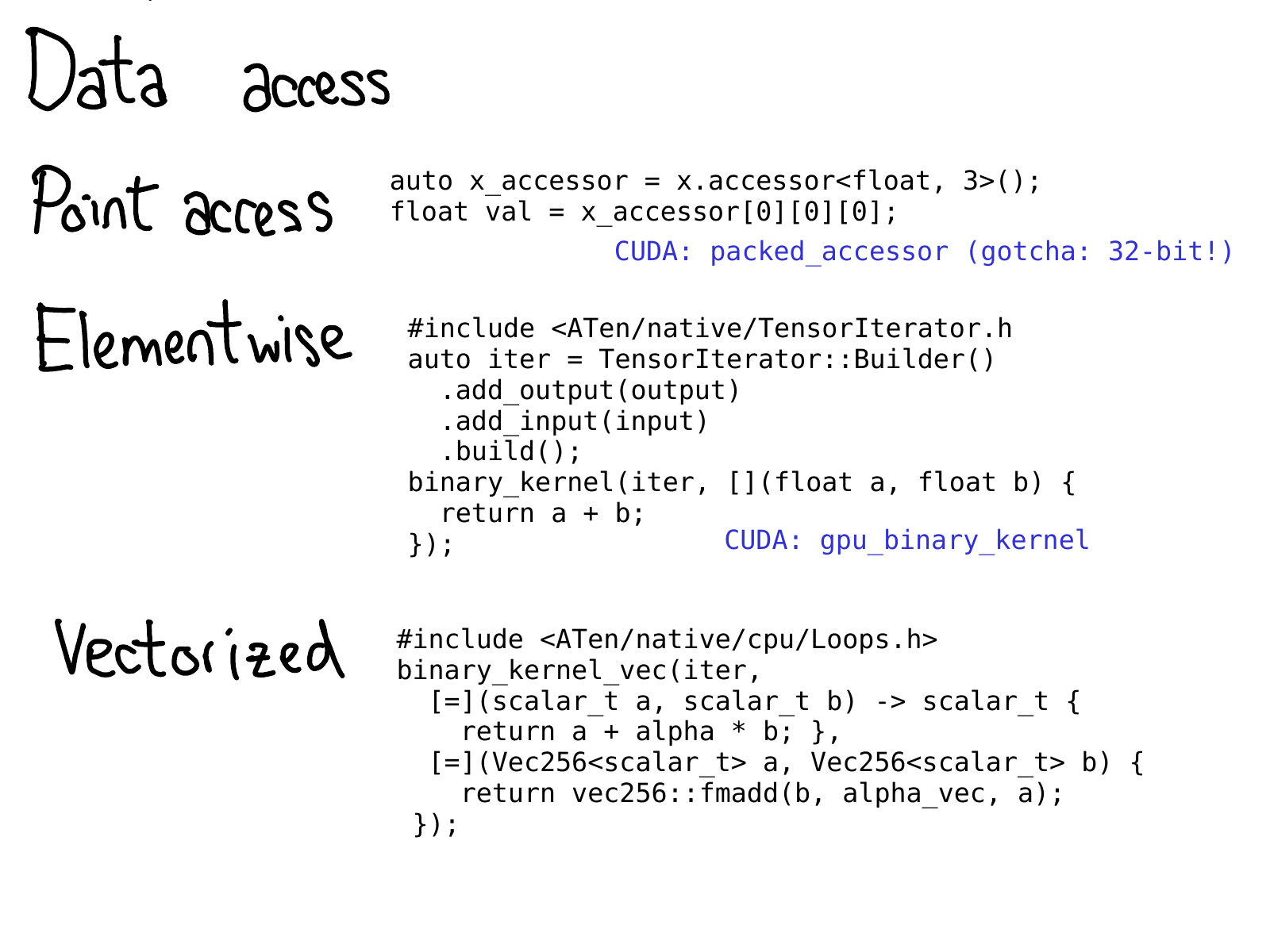
At some point, we have to actually access the data. PyTorch offers quite a few options for doing this.

1. If you just want to get a value at some specific location, you should use TensorAccessor. A tensor accessor is like a tensor, but it hard codes the dimensionality and dtype of the tensor as template parameters. When you retrieve an accessor like x.accessor<float, 3>();, we do a runtime test to make sure that the tensor really is this format; but after that, every access is unchecked. Tensor accessors handle strides correctly, so you should prefer using them over raw pointer access (which, unfortunately, some legacy kernels do.) There is also a PackedTensorAccessor, which is specifically useful for sending an accessor over a CUDA launch, so that you can get accessors from inside your CUDA kernel. (One notable gotcha: TensorAccessor defaults to 64-bit indexing, which is much slower than 32-bit indexing in CUDA!)
2. If you're writing some sort of operator with very regular element access, for example, a pointwise operation, you are much better off using a higher level of abstraction, the TensorIterator. This helper class automatically handles broadcasting and type promotion for you, and is quite handy.
3. For true speed on CPU, you may need to write your kernel using vectorized CPU instructions. We've got helpers for that too! The Vec256 class represents a vector of scalars and provides a number of methods which perform vectorized operations on them all at once. Helpers like binary_kernel_vec then let you easily run vectorized operations, and then finish everything that doesn't round nicely into vector instructions using plain old instructions. The infrastructure here also manages compiling your kernel multiple times under different instruction sets, and then testing at runtime what instructions your CPU supports, and using the best kernel in those situations.

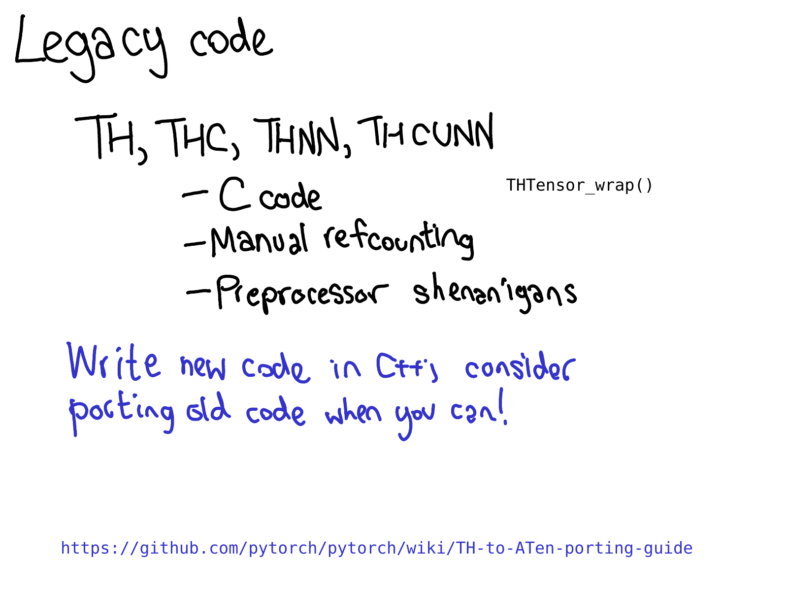
A lot of kernels in PyTorch are still written in the legacy TH style. (By the way, TH stands for TorcH. It's a pretty nice acronym, but unfortunately it is a bit poisoned; if you see TH in the name, assume that it's legacy.) What do I mean by the legacy TH style?

1. It's written in C style, no (or very little) use of C++.
2. It's manually refcounted (with manual calls to THTensor_free to decrease refcounts when you're done using tensors), and
3. It lives in generic/ directory, which means that we are actually going to compile the file multiple times, but with different #define scalar_t.

This code is pretty crazy, and we hate reviewing it, so please don't add to it. One of the more useful tasks that you can do, if you like to code but don't know too much about kernel writing, is to port some of these TH functions to ATen.

---

To wrap up, I want to talk a little bit about working efficiently on PyTorch. If the largeness of PyTorch's C++ codebase is the first gatekeeper that stops people from contributing to PyTorch, the efficiency of your workflow is the second gatekeeper. If you try to work on C++ with Python habits, you will have a bad time: it will take forever to recompile PyTorch, and it will take you forever to tell if your changes worked or not.

How to work efficiently could probably be a talk in and of itself, but this slide calls out some of the most common anti-patterns I've seen when someone complains: "It's hard to work on PyTorch."

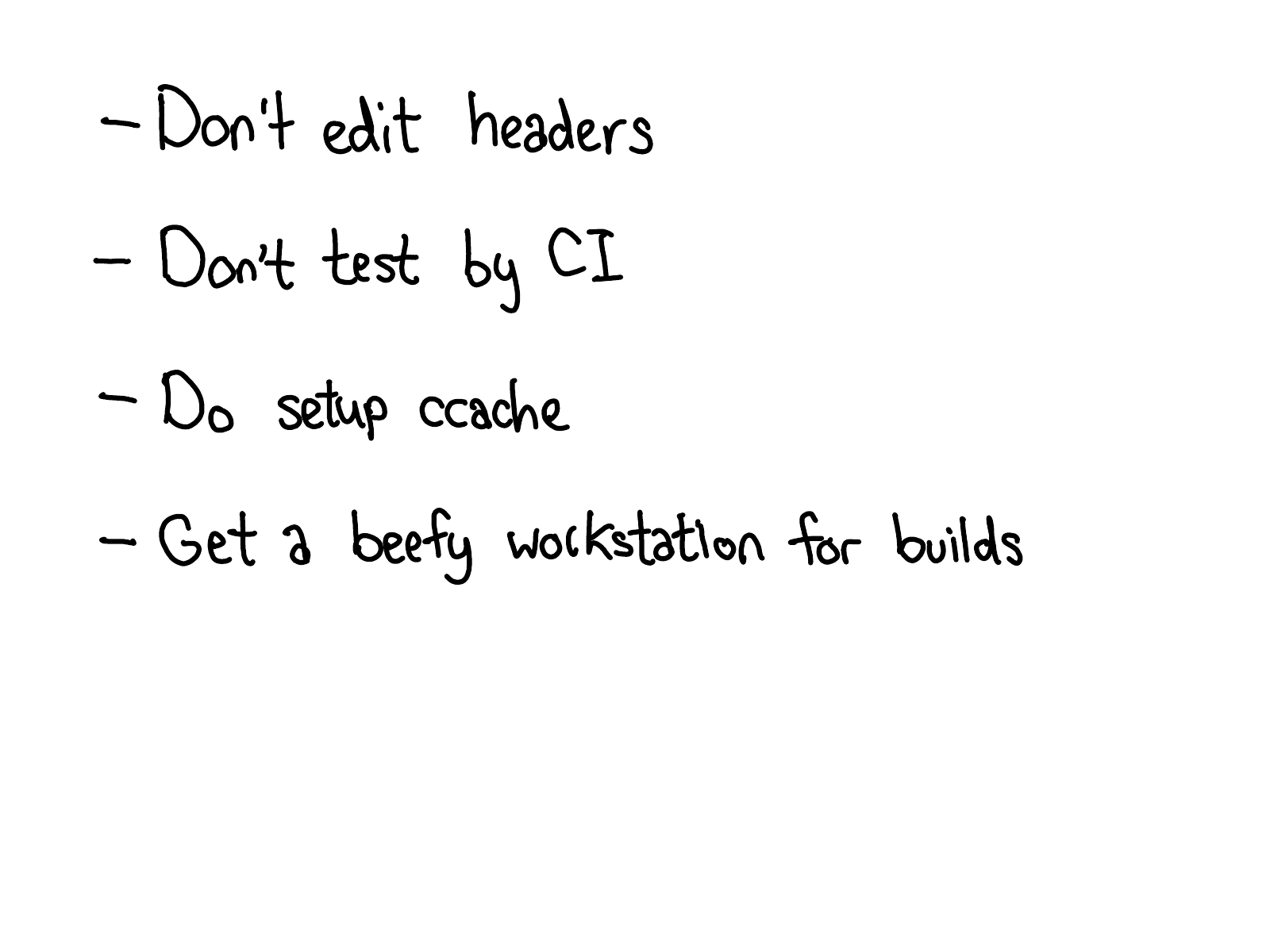
1. If you edit a header, especially one that is included by many source files (and especially if it is included by CUDA files), expect a very long rebuild. Try to stick to editing cpp files, and edit headers sparingly!
2. Our CI is a very wonderful, zero-setup way to test if your changes worked or not. But expect to wait an hour or two before you get back signal. If you are working on a change that will require lots of experimentation, spend the time setting up a local development environment. Similarly, if you run into a hard to debug problem on a specific CI configuration, set it up locally. You can download and run the Docker images locally
3. The CONTRIBUTING guide explains how to setup ccache; this is highly recommended, because sometimes it will help you get lucky and avoid a massive recompile when you edit a header. It also helps cover up bugs in our build system, when we recompile files when we shouldn't.
4. At the end of the day, we have a lot of C++ code, and you will have a much more pleasant experience if you build on a beefy server with CPUs and RAM. In particular, I don't recommend doing CUDA builds on a laptop; building CUDA is sloooooow and laptops tend to not have enough juice to turnaround quickly enough.

---

So that's it for a whirlwind tour of PyTorch's internals! Many, many things have been omitted; but hopefully the descriptions and explanations here can help you get a grip on at least a substantial portion of the codebase.

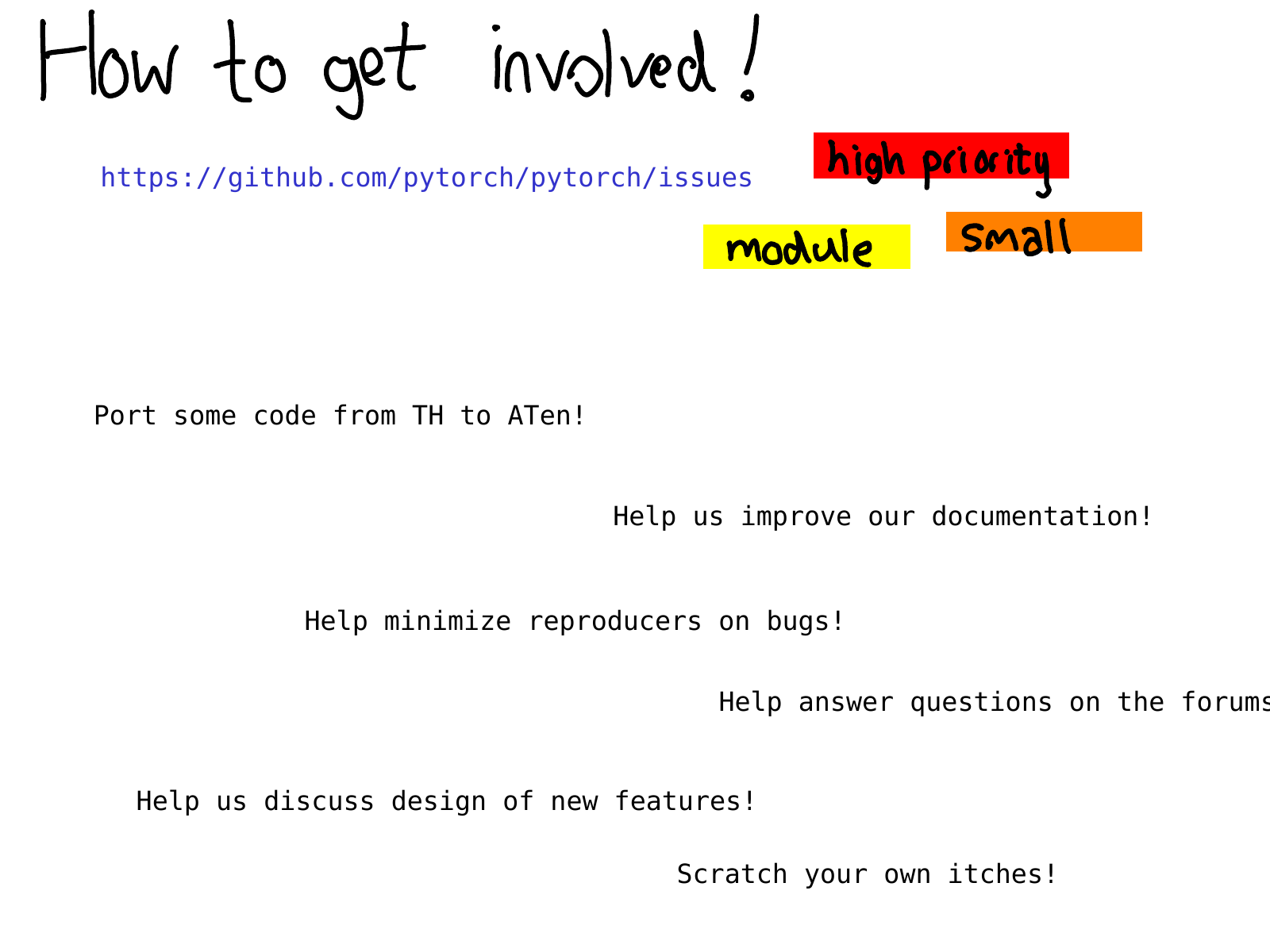
Where should you go from here? What kinds of contributions can you make? A good place to start is our issue tracker. Starting earlier this year, we have been triaging issues; issues labeled triaged mean that at least one PyTorch developer has looked at it and made an initial assessment about the issue. You can use these labels to find out what issues we think are high priority or look up issues specific to some module, e.g., autograd or find issues which we think are small (word of warning: we're sometimes wrong!)

Even if you don't want to get started with coding right away, there are many other useful activities like improving documentation (I love merging documentation PRs, they are so great), helping us reproduce bug reports from other users, and also just helping us discuss RFCs on the issue tracker. PyTorch would not be where it is today without our open source contributors; we hope you can join us too!

Some notes collected from a close read of Conal Elliot's Compiling to Categories and The Simple Essence of Automatic Differentiation.

A colleague of mine was trying to define a "tree structure" of tensors, with the hope of thereby generalizing the concept to also work with tensors that have "ragged dimensions." Let's take a look:

Suppose we have a (2, 3) matrix:

tensor([[1, 2, 3],
        [4, 5, 6]])

One way to think about this is that we have a "tree" of some sort, where the root of the tree branches to two subnodes, and then each subnode branches to three nodes:

       /- ROOT -\
  ROW 1          ROW 2
 /  |  \        /  |  \
1   2   3      4   5   6

Suppose you wanted to define this data structure in Haskell. One obvious way of going about doing this is to just say that a matrix is just a bunch of nested lists, [[Float]]. This works, true, but it isn't very illuminating, and it is certainly not type safe. Type safety could be achieved with sized vectors, but we are still left wondering, "what does it mean?"

Often, inductive definitions fall out of how we compose things together, in the same way that the inductive data structure for a programming language tells us how we take smaller programs and put them together to form a larger program. With matrices, we can think of a pictorial way of composing them, by either attaching matrices together vertically or horizontally. That gives us this vocabulary for putting together matrices, which would let us (non-uniquely) represent every matrix (Compiling to Categories, Section 8):

data Matrix
  = Scalar Float
  | Horizontal Matrix Matrix
  | Vertical Matrix Matrix

But what does it mean? Well, every matrix represents a linear map (if A : (n, m) is your matrix, the linear map is the function R^m -> R^n, defined to be f(x) = A x. We'll call a linear map from a to b, Linear a b). So the question we ask now is, what does it mean to "paste" two matrices together? It's a way of composing two linear maps together into a new linear map:

-- A function definition does not a category make!  You have to
-- prove that the resulting functions are linear.

horizontal :: Linear a c -> Linear b c -> Linear (a, b) c
horizontal f g = \(a, b) -> f a + g b

-- In matrix form:
--
--              [ a ]
-- [ F  |  G ]  [ - ] = [ F a + G b ]
--              [ b ]

vertical :: Linear a c -> Linear a d -> Linear a (c, d)
vertical f g = \a -> (f a, g a)

-- In matrix form:
--
-- [ F ]         [ F a ]
-- [ - ] [ a ] = [  -  ]
-- [ G ]         [ G a ]

Now we're cooking! Notice that the pasting shows up in the type of the linear map: if we paste horizontally, that just means that the vectors this linear map takes in have to be pasted together (with the tuple constructor); similarly, if we paste vertically, we'll produce output vectors that are the pasted results.

Cool, so we can add some type indexes, and write Linear as a GADT to refine the indices when you apply the constructor:

data Linear a b where
  Scalar :: Float -> Linear Float Float
  Horizontal :: Linear a c -> Linear b c -> Linear (a, b) c
  Vertical :: Linear a c -> Linear a d -> Linear a (c, d)

Is this the end of the story? Not quite. There are many ways you can go about combining linear maps; for example, you could (literally) compose two linear maps together (in the same sense of function composition). It's true that you can paste together any matrix you like with the data type above; how do we decide what should and shouldn't go in our language of linear maps?

To this end, Conal Elliot calls on the language of category theory to adjudicate. A category should define identity and function composition:

identity :: Linear a a
identity a = a

-- In matrix form: the identity matrix

compose :: Linear b c -> Linear a b -> Linear a c
compose g f = \a -> g (f a)

-- In matrix form: matrix multiply

We find that Horizontal and Vertical are the elimination and introduction operations of cocartesian and cartesian categories (respectively).

But this should we just slap Identity and Compose constructors to our data type? Linear map composition is a computationally interesting operation: if we just keep it around as syntax (rather than doing what is, morally, a matrix multiply), then it will be quite expensive to do operations on the final linear map. Where do representable functors come in? I'm not exactly sure how to explain this, and I've run out of time for this post; stay tuned for a follow up.

Long time readers of mine may be aware that I used a ThinkPad X61T for the past decade. After the hinge on my second instance of the machine, I decided it was finally time to get a new laptop. And I had one particular model on my eye, after Simon Peyton Jones showed me his new laptop at the last Haskell Implementor's Workshop: the Microsoft Surface Book 2. It fits my primary requirement for a laptop: it's a convertible laptop into tablet mode with a digitizer pen. The pen is not Wacom branded but it has an eraser end and can magnetically attach to the laptop (no enclosure for the pen, but I think that for modern hardware that constraint is unsatisfiable.) Furthermore, there is a Linux enthusiast community around the device, which made me feel that it would be more likely I could get Linux to work. So a few weeks ago, I took the plunge, and laid down three grand for my own copy. It has worked out well, but in the classic Linux style, not without a little bit of elbow grease.

It's been a year since I got my hood and gown and joined Facebook (where I've been working on PyTorch), but while I've been at Facebook Backpack hasn't been sleeping; in fact, there's been plenty of activity, more than I could have ever hoped for. I wanted to summarize some of the goings on in this blog post.