Hoopl: Dataflow lattices
April 4, 2011The essence of dataflow optimization is analysis and transformation, and it should come as no surprise that once you’ve defined your intermediate representation, the majority of your work with Hoopl will involve defining analysis and transformations on your graph of basic blocks. Analysis itself can be further divided into the specification of the dataflow facts that we are computing, and how we derive these dataflow facts during analysis. In part 2 of this series on Hoopl, we look at the fundamental structure backing analysis: the dataflow lattice. We discuss the theoretical reasons behind using a lattice and give examples of lattices you may define for optimizations such as constant propagation and liveness analysis.
Despite its complicated sounding name, dataflow analysis remarkably resembles the way human programmers might reason about code without actually running it on a computer. We start off with some initial belief about the state of the system, and then as we step through instructions we update our belief with new information. For example, if I have the following code:
f(x) {
  a = 3;
  b = 4;
  return (x * a + b);
}
At the very top of the function, I don’t know anything about x. When I see the expressions a = 3 and b = 4, I know that a is equal to 3 and b is equal to 4. In the least expression, I could use constant propagation to simplify the result to x * 3 + 4. Indeed, in the absence of control flow, we can think of analysis simply as stepping through the code line by line and updating our assumptions, also called dataflow facts. We can do this in both directions: the analysis we just did above was forwards analysis, but we can also do backwards analysis, which is the case for liveness analysis.
Alas, if only things were this simple! There are two spanners in the works here: Y-shaped control flows and looping control flows.
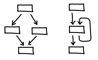
Y-shaped control flows (called joins, for both obvious reasons and reasons that will become clear soon) are so named because there are two, distinct paths of execution that then merge into one. We then have two beliefs about the state of the program, which we need to reconcile before carrying on:
f(x) {
  if (x) {
    a = 2; // branch A
  } else {
    a = 3; // branch B
  }
  return a;
}
Inside branch A, we know that a is 2, and inside branch B, we know a is 3, but outside this conditional, all we can say is that a is either 2 or 3. (Since two possible values isn’t very useful for constant propagation, we’ll instead say the value of a is top: there is no one value that represents the value held at a.) The upshot is that any set of dataflow facts you are doing analysis with must have a join operation defined:
data DataflowFactsTry1 a = DF1 { fact_join :: a -> a -> a }
There is an analogous situation for backwards analysis, which occurs when you have a conditional jump: two “futures” of the control flow join back together, and so a similar join needs to occur.
Looping control flows also have joins, but they have the further problem that we don’t know what one of the incoming code path’s state is: we can’t figure it out until we’ve analyzed the loop body, but to analyze the loop body, we need to know what the incoming state is. It’s a Catch-22! The trick to work around this is to define a bottom fact, which intuitively represents the most conservative dataflow fact possible: it is the identity when joined some other dataflow fact. So when we encounter one of these loop edges, instead of attempting to calculate the edge (which is a Catch-22 problem), we instead feed in the bottom element, and get an approximation of what the fact at that loop edge is. If this approximation is better than bottom, we feed the new result in instead, and the process repeats until there are no more changes: a fixpoint has been achieved.
With join and bottom in hand, the mathematically inclined may notice that what we’ve defined looks a lot like a lattice:
data DataflowLattice a = DataflowLattice
 { fact_name       :: String          -- Documentation
 , fact_bot        :: a               -- Lattice bottom element
 , fact_join       :: JoinFun a       -- Lattice join plus change flag
                                      -- (changes iff result > old fact)
 }
type JoinFun a = Label -> OldFact a -> NewFact a -> (ChangeFlag, a)
There is a little bit of extra noise in here: Label is included strictly for debugging purposes (it tells the join function what label the join is occurring on) and ChangeFlag is included for optimization purposes: it lets fact_join efficiently say when the fixpoint has been achieved: NoChange.
Aside: Lattices. Here, we review some basic terminology and intuition for lattices. A lattice is a partially ordered set, for which least upper bounds (lub) and greatest lower bounds (glb) exist for all pairs of elements. If one imagines a Hasse diagram, the existence of a least upper bound means that I can follow the diagram upwards from two elements until I reach a shared element; the greatest least bound is the same process downwards. The least upper bound is also called the join of two elements, and the greatest least bound the meet. (I prefer lub and glb because I always mix join and meet up!) Notationally, the least upper bound is represented with the logical or symbol or a square union operator, while the greatest least bound is represented with the logical and symbol or square intersection operator. The choice of symbols is suggestive: the overloading of logical symbols corresponds to the fact that logical propositions can have their semantics defined using a special kind of lattice called a boolean algebra, where lub is equivalent to or and glb is equivalent to and (bottom is falsity and top is tautology). The overloading of set operators corresponds to the lattice on the usual ordering of the powerset construction: lub is set union and glb is set intersection.
In Hoopl, we deal with bounded lattices, lattices for which a top and bottom element exist. These are special elements that are greater than and less than (respectively) than all other elements. Joining the bottom element with any other element is a no-op: the other element is the result (this is why we use bottom as our initialization value!) Joining the top element with any other element results in the top element (thus, if you get to the top, you’re “stuck”, so to speak).
For the pedantic, strictly speaking, Hoopl doesn’t need a lattice: instead, we need a bounded semilattice (since we only require joins, and not meets, to be defined.) There is another infelicity: the Lerner-Grove-Chambers and Hoopl uses bottom and join, but most of the existing literature on dataflow lattices uses top and meet (essentially, flip the lattice upside down.) In fact, which choice is “natural” depends on the analysis: as we will see, liveness analysis naturally suggests using bottom and join, while constant propagation suggests using top and meet. To be consistent with Hoopl, we’ll use bottom and join consistently; as long as we’re consistent, the lattice orientation doesn’t matter.
We will now look at concrete examples of using the dataflow lattices for liveness analysis and constant propagation. These two examples give a nice spread of lattices to look at: liveness analysis is a set of variable names, while constant propagation is a map of variable names to a flat lattice of possible values.
Liveness analysis (Live.hs) uses a very simple lattice, so it serves as a good introductory example for the extra ceremony that is involved in setting up a DataflowLattice:
type Live = S.Set Var
liveLattice :: DataflowLattice Live
liveLattice = DataflowLattice
  { fact_name = "Live variables"
  , fact_bot  = S.empty
  , fact_join = add
  }
    where add _ (OldFact old) (NewFact new) = (ch, j)
            where
              j = new `S.union` old
              ch = changeIf (S.size j > S.size old)
The type Live is the type of our data flow facts. This represents is the set of variables that are live (that is, will be used by later code):
f() {
  // live: {x, y}
  x = 3;
  y = 4;
  y = x + 2;
  // live: {y}
  return y;
  // live: {}
}
Remember that liveness analysis is a backwards analysis: we start at the bottom of our procedure and work our way up: a usage of a variable means that it’s live for all points above it. We fill in DataflowLattice with documentation, the distinguished element (bottom) and the operation on these facts (join). Var is Expr.hs and simply is a string name of the variable. Our bottom element (which is used to initialize edges that we can’t calculate right off the bat) is the empty set, since at the bottom of any procedure, all variables are dead.
Join is set union, which can be clearly seen in this example:
f (x) {
  // live: {a,b,x,r} (union of the two branches,
  // as well as x, due to its usage in the conditional)
  a = 2;
  b = 3;
  if (x) {
    // live: {a,r}
    r = a;
  } else {
    // live: {b,r}
    r = b;
  }
  // live: {r}
  return r;
  // live: {}
}
We also see some code for calculating the change ch, which is a simple size comparison of sets, because union will only ever increase the size of a set, not decrease it. changeIf is a utility function that takes Bool to ChangeFlag.
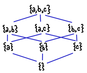
Here is an illustration of the lattice structure if we have three variables: it’s simply the usual ordering on the powerset construction.
Here is the lattice for constant propagation (ConstProp.hs). It is slightly more complicated than the live set, though some of the complexity is hidden by the fact that Hoopl provides some utility data types and functions:
-- ConstFact:
--   Not present in map => bottom
--   PElem v => variable has value v
--   Top     => variable's value is not constant
type ConstFact = Map.Map Var (WithTop Lit)
constLattice :: DataflowLattice ConstFact
constLattice = DataflowLattice
 { fact_name = "Const var value"
 , fact_bot  = Map.empty
 , fact_join = joinMaps (extendJoinDomain constFactAdd) }
 where
   constFactAdd _ (OldFact old) (NewFact new)
       = if new == old then (NoChange, PElem new)
         else               (SomeChange, Top)
There are essentially two lattices in this construction. The “outer” lattice is the map, for which the bottom element is the empty map and the join is joining two maps together, merging elements using the inner lattice. The “inner” (semi)lattice is WithTop Lit, which is provided by Hoopl. (One may say that the inner lattice is pointwise lifted into the map.) We illustrate the inner lattice here for variables containing booleans:
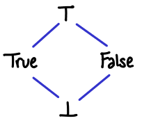
One thing to stress about the inner lattice is the difference between bottom and top. Both represent a sort of “not knowing about the contents of a variable”, but in the case of bottom, the variable may be constant or it may not be constant, whereas in top, the variable is definitely not constant. It is easy to get tripped up saying things like, “bottom means that we don’t know what the value of the variable is” and “top means that the value of the variable could be anything.” If we think of this lattice as a set, with {True} indicating that the value of this variable is true, then {True,False} (bottom) indicates the variable could be a constant true or constant false, not that the variable could be true or false. This also means we can interpret {} (top) appropriately: there is no value for which this variable is a constant. (Notice that this is the powerset lattice flipped upside down!)
There are a few interesting utility functions in this example: extendJoinDomain and joinMaps. extendJoinDomain saves us the drudgery from having to write out all of the interactions with top in full, e.g.:
constFactAddExtended _ (OldFact old) (NewFact new)
   = case (old, new) of
        (Top, _) -> (NoChange, Top)
        (_, Top) -> (SomeChange, Top)
        (PElem old, PElem new) | new == old -> (NoChange, PElem new)
                               | otherwise -> (SomeChange, Top)
joinMaps lifts our inner lattice into map form, and also takes care of the ChangeFlag plumbing (output SomeChange if any entry in the new map wasn’t present in the old map, or if any of the joined entries changed).
That concludes our discussion of Hoopl and dataflow lattices. We haven’t covered all of the functions Hoopl provides to manipulate dataflow lattices; here are some further modules to look at:
Compiler.Hoopl.CombinatorsdefinespairLattice, which takes the product construction of two lattices. It can be used to easily perform multiple analyses at the same time.Compiler.Hoopl.Pointeddefines a number of auxiliary data structures and functions for addingTopandBottomto existing data types. This is whereextendJoinDomaincomes from.Compiler.Hoopl.CollectionsandCompiler.Hoopl.Uniquedefine maps and sets on unique keys (most prominently, labels). You will most probably be using these for your dataflow lattices.
Next time, we will talk about transfer functions, the mechanism by which we calculate dataflow facts.
Further reading. Dataflow lattices are covered in chapter 10.11 of Compilers: Principles, Techniques and Tools (the Red Dragon Book). The original paper was Kildall’s 1973 paper A unified approach to global program optimization. Interestingly enough, the Dragon Book remarks that “it has not seen widespread use, probably because the amount of labor saved by the system is not as great as that saved by tools like parser generators.” My feeling is that this is the case for traditional compiler optimization passes, but not for Lerner-Grove-Chambers style passes (where analysis and rewriting are interleaved.)
It’s worth noting that the definition given for liveness is a simplification of the traditional definition, which both adds and removes variables from the live set. It’s not wrong, just less precise (it can’t remove the redundant store y = 4 in the first example):
f() { // live: {} x = 3; // live: {x} y = 4; // live: {x} y = x + 2; // live: {y} return y; // live: {} }
Thanks for the post. One quibble: It’s “greatest lower bound,” not “greatest least bound.”
(Also, as Ben Karel correctly points out, what you’re calling liveness really isn’t, so maybe you should call it something else. It probably makes sense to present transfer functions before the lattice, since you can make examples for straight-line code with just transfer functions, but you can’t make legit examples with just the lattice.)
Thanks, fixed the glb bit!
Do you know if there’s a standard name for the less precise “liveness” analysis? The remark about presenting transfer functions before the lattice is also well taken. Probably the best approach is to introduce the type of facts, give examples of transfer functions, and then introduce the lattice structure.