ezyang’s blog

Once you’ve determined what dataflow facts you will be collecting, the next step is to write the transfer function that actually performs this analysis for you!

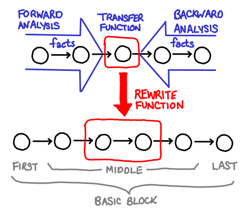
Remember what your dataflow facts mean, and this step should be relatively easy: writing a transfer function usually involves going through every possible statement in your language and thinking about how it changes your state. We’ll walk through the transfer functions for constant propagation and liveness analysis.

---

Here is the transfer function for liveness analysis (once again, in Live.hs):

liveness :: BwdTransfer Insn Live
liveness = mkBTransfer live
  where
    live :: Insn e x -> Fact x Live -> Live
    live   (Label _)       f = f
    live n@(Assign x _)    f = addUses (S.delete x f) n
    live n@(Store _ _)     f = addUses f n
    live n@(Branch l)      f = addUses (fact f l) n
    live n@(Cond _ tl fl)  f = addUses (fact f tl `S.union` fact f fl) n
    live n@(Call vs _ _ l) f = addUses (fact f l `S.difference` S.fromList vs) n
    live n@(Return _)      _ = addUses (fact_bot liveLattice) n

    fact :: FactBase (S.Set Var) -> Label -> Live
    fact f l = fromMaybe S.empty $ lookupFact l f

    addUses :: S.Set Var -> Insn e x -> Live
    addUses = fold_EN (fold_EE addVar)
    addVar s (Var v) = S.insert v s
    addVar s _       = s

live is the meat of our transfer function: it takes an instruction and the current fact, and then modifies the fact in light of that information. Because this is a backwards transfer (BwdTransfer), the Fact x Live passed to live are the dataflow facts after this instruction, and our job is to calculate what the dataflow facts are before the instruction (the facts flow backwards).

If you look closely at this function, there’s something rather curious going on: in the line live (Label _) f = f, we simply pass out f (which ostensibly has type Fact x Live) as the result. How does that work? Well, Fact is actually a type family:

type family   Fact x f :: *
type instance Fact C f = FactBase f
type instance Fact O f = f

Look, it’s the O and C phantom types again! If we recall our definition of Insn (in IR.hs):

data Insn e x where
  Label  :: Label  ->                               Insn C O
  Assign :: Var    -> Expr    ->                    Insn O O
  Store  :: Expr   -> Expr    ->                    Insn O O
  Branch :: Label  ->                               Insn O C
  Cond   :: Expr   -> Label   -> Label  ->          Insn O C
  Call   :: [Var]  -> String  -> [Expr] -> Label -> Insn O C
  Return :: [Expr] ->                               Insn O C

That means for any of the instructions that are open on exit (x = O for Label, Assign and Store), our function gets Live, whereas for an instruction that is closed on exit (x = C for Branch, Cond, Call and Return), we get FactBase Live, which is a map of labels to facts (LabelMap Live)—for reasons we will get to in a second.

Because the type of our arguments actually change depending on what instruction we receive, some people (GHC developers among them) prefer to use the long form mkBTransfer3, which takes three functions, one for each shape of node. The rewritten code thus looks like this:

liveness' :: BwdTransfer Insn Live
liveness' = mkBTransfer3 firstLive middleLive lastLive
  where
    firstLive :: Insn C O -> Live -> Live
    firstLive (Label _) f = f

    middleLive :: Insn O O -> Live -> Live
    middleLive n@(Assign x _) f = addUses (S.delete x f) n
    middleLive n@(Store _ _)  f = addUses f n

    lastLive :: Insn O C -> FactBase Live -> Live
    lastLive n@(Branch l)      f = addUses (fact f l) n
    lastLive n@(Cond _ tl fl)  f = addUses (fact f tl `S.union` fact f fl) n
    lastLive n@(Call vs _ _ l) f = addUses (fact f l `S.difference` S.fromList vs) n
    lastLive n@(Return _)      _ = addUses (fact_bot liveLattice) n

(with the same definitions for fact, addUses and addVar).

With this in mind, it should be fairly easy to parse the code for firstLive and middleLive. Labels don’t change the set of live libraries, so our fact f is passed through unchanged. For assignments and stores, any uses of a register in that expression makes that register live (addUses is a utility function that calculates this), but if we assign to a register, we lose its previous value, so it is no longer live. Here is some pseudocode demonstrating:

// a is live
x = a;
// a is not live
foo();
// a is not live
a = 2;
// a is live
y = a;

If you’re curious out the implementation of addUses, the fold_EE and fold_EN functions can be found in OptSupport.hs:

fold_EE :: (a -> Expr -> a) -> a -> Expr      -> a
fold_EN :: (a -> Expr -> a) -> a -> Insn e x -> a

fold_EE f z e@(Lit _)         = f z e
fold_EE f z e@(Var _)         = f z e
fold_EE f z e@(Load addr)     = f (f z addr) e
fold_EE f z e@(Binop _ e1 e2) = f (f (f z e2) e1) e

fold_EN _ z (Label _)       = z
fold_EN f z (Assign _ e)    = f z e
fold_EN f z (Store addr e)  = f (f z e) addr
fold_EN _ z (Branch _)      = z
fold_EN f z (Cond e _ _)    = f z e
fold_EN f z (Call _ _ es _) = foldl f z es
fold_EN f z (Return es)     = foldl f z es

The naming convention is as follows: E represents an Expr, while N represents a Node (Insn). The left letter indicates what kind of values are passed to the combining function, while the right letter indicates what is being folded over. So fold_EN folds all Expr in a Node and calls the combining function on it, while fold_EE folds all of the Expr inside an Expr (notice that things like Load and Binop can contain expressions inside themselves!) The effect of fold_EN (fold_EE f), then, is that f will be called on every expression in a node, which is exactly what we want if we’re checking for uses of Var.

We could have also written out the recursion explicitly:

addUses :: S.Set Var -> Insn e x -> Live
addUses s (Assign _ e)      = expr s e
addUses s (Store e1 e2)     = expr (expr s e1) e2
addUses s (Cond e _ _)      = expr s e
addUses s (Call _ _ es _)   = foldl expr s es
addUses s (Return es)       = foldl expr s es
addUses s _                 = s

expr :: S.Set Var -> Expr -> Live
expr s e@(Load e') = addVar (addVar s e) e'
expr s e@(Binop _ e1 e2) = addVar (addVar (addVar s e) e1) e2
expr s e = addVar s e

But as you can see, there’s a lot of junk involved with recursing down the structure, and you might accidentally forget an Expr somewhere, so using a pre-defined fold operator is preferred. Still, if you’re not comfortable with folds over complicated datatypes, writing out the entire thing in full at least once is a good exercise.

The last part to look at is lastLives:

lastLive :: Insn O C -> FactBase Live -> Live
lastLive n@(Branch l)      f = addUses (fact f l) n
lastLive n@(Cond _ tl fl)  f = addUses (fact f tl `S.union` fact f fl) n
lastLive n@(Call vs _ _ l) f = addUses (fact f l `S.difference` S.fromList vs) n
lastLive n@(Return _)      _ = addUses (fact_bot liveLattice) n

There are several questions to ask.

1. Why does it receive a FactBase Live instead of a Live? This is because, as the end node in a backwards analysis, we may receive facts from multiple locations: each of the possible paths the control flow may go down.

   In the case of a Return, there are no further paths, so we use fact_bot liveLattice (no live variables). In the case of Branch and Call, there is only one further path l (the label we’re branching or returning to), so we simply invoke fact f l. And finaly, for Cond there are two paths: tl and fl, so we have to grab the facts for both of them and combine them with what happens to be our join operation on the dataflow lattice.

2. Why do we still need to call addUses? Because instructions at the end of basic blocks can use variables (Cond may use them in its conditional statement, Return may use them when specifying what it returns, etc.)

3. What’s with the call to S.difference in Call? Recall that vs is the list of variables that the function call writes its return results to. So we need to remove those variables from the live variable set, since they will get overwritten by this instruction:

   f (x, y) {
   L100:
     goto L101
   L101:
     if x > 0 then goto L102 else goto L104
   L102:
     // z is not live here
     (z) = f(x-1, y-1) goto L103
   L103:
     // z is live here
     y = y + z
     x = x - 1
     goto L101
   L104:
     ret (y)
   }
   

You should already have figured out what fact does: it looks up the set of dataflow facts associated with a label, and returns an empty set (no live variables) if that label isn’t in our map yet.

---

Once you’ve seen one Hoopl analysis, you’ve seen them all! The transfer function for constant propagation looks very similar:

-- Only interesting semantic choice: values of variables are live across
-- a call site.
-- Note that we don't need a case for x := y, where y holds a constant.
-- We can write the simplest solution and rely on the interleaved optimization.
--------------------------------------------------
-- Analysis: variable equals a literal constant
varHasLit :: FwdTransfer Node ConstFact
varHasLit = mkFTransfer ft
 where
  ft :: Node e x -> ConstFact -> Fact x ConstFact
  ft (Label _)            f = f
  ft (Assign x (Lit k))   f = Map.insert x (PElem k) f
  ft (Assign x _)         f = Map.insert x Top f
  ft (Store _ _)          f = f
  ft (Branch l)           f = mapSingleton l f
  ft (Cond (Var x) tl fl) f
      = mkFactBase constLattice
           [(tl, Map.insert x (PElem (Bool True))  f),
            (fl, Map.insert x (PElem (Bool False)) f)]
  ft (Cond _ tl fl) f
      = mkFactBase constLattice [(tl, f), (fl, f)]
  ft (Call vs _ _ bid)      f = mapSingleton bid (foldl toTop f vs)
      where toTop f v = Map.insert v Top f
  ft (Return _)             _ = mapEmpty

The notable difference is that, unlike liveness analysis, constant propagation analysis is a forward analysis FwdTransfer. This also means the type of the function is Node e x -> f -> Fact x f, rather than Node e x -> Fact x f -> f: when the control flow splits, we can give different sets of facts for the possible outgoing labels. This is used to good effect in Cond (Var x), where we know that if we take the first branch the condition variable is true, and vice-versa. The rest is plumbing:

• Branch: An unconditional branch doesn’t cause any of our variables to stop being constant. Hoopl will automatically notice if a different path to that label has contradictory facts and convert the mappings to Top as notice, using our lattice’s join function. mapSingleton creates a singleton map from the label l to the fact f.
• Cond: We need to create a map with two entries, which is can be done conveniently with mkFactBase, where the last argument is a list of labels to maps.
• Call: A function call is equivalent to assigning lots of unknown variables to all of its return variables, so we set all of them to unknown with toTop.
• Return: Goes nowhere, so an empty map will do.

Next time, we’ll talk about some of the finer subtleties about transfer functions and join functions, and discuss graph rewriting, and wrap it all up with some use of Hoopl’s debugging facilities to observe how Hoopl rewrites a graph.