Getting a fix on fixpoints
Previously, we’ve drawn Hasse diagrams of all sorts of Haskell types, from data types to function types, and looked at the relationship between computability and monotonicity. In fact, all computable functions are monotonic, but not all monotonic functions are computable. Is there some description of functions that entails computability? Yes: Scott continuous functions. In this post, we look at the mathematical machinery necessary to define continuity. In particular, we will look at least upper bounds, chains, chain-complete partial orders (CPOs) and domains. We also look at fixpoints, which arise naturally from continuous functions.
In our previous diagrams of types with infinitely many values, we let the values trail off into infinity with an ellipsis.
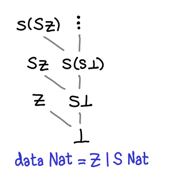
As several commentors have pointed out, this is not quite right: all Haskell data types also have a one or more top values, values that are not less than any other value. (Note that this is distinct from values that are greater than or equal to all other values: some values are incomparable, since these are partial orders we’re talking about.) In the case of Nat, there are a number of top values: Z, S Z, S (S Z), and so on are the most defined you can get. However, there is one more: fix S, aka infinity.
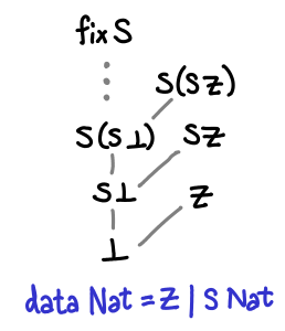
There are no bottoms lurking in this value, but it does seem a bit odd: if we peel off an S constructor (decrement the natural number), we get back fix S again: infinity minus one is apparently infinity.
In fact, fix S is a least upper bound for the chain ⊥, S ⊥, S (S ⊥)... A chain is simply a sequence of values for which d_1 ≤ d_2 ≤ d_3 ...; they are lines moving upwards on the diagrams we’ve drawn.
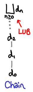
The least upper bound of a chain is just a value d which is bigger than all the members of the chain: it “sits at the top.” (For all n > 0, d_n ≤ d.) It is notated with a |_|, which is frequently called the “lub” operator. If the chain is strictly increasing, the least upper bound cannot be in the chain, because if it were, the next element in the chain would be greater than it.
A chain in a poset may not necessarily have a least upper bound. Consider the natural numbers with the usual partial ordering.
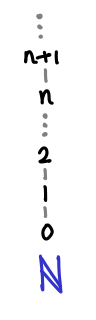
The chain 0 ≤ 1 ≤ 2 ≤ ... does not have an upper bound, because the set of natural numbers doesn’t contain an infinity. We have to instead turn to Ω, which is the natural numbers and the smallest possible infinity, the ordinal ω.
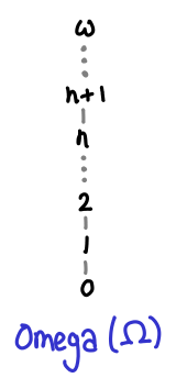
Here the chain has a least upper bound.
Despite not having a lub for 0 ≤ 1 ≤ 2 ≤ ..., the natural numbers have many least upper bounds, since every element n forms the trivial chain n ≤ n ≤ n...
Here are pictorial representatios of some properties of lubs.
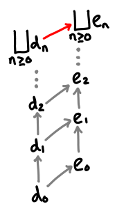
If one chain is always less than or equal to another chain, that chain’s lub is less than or equal to the other chain’s lub.
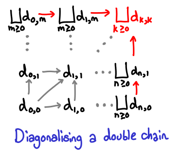
A double chain of lubs works the way you expect it to; furthermore, we can diagonalize this chain to get the upper bound in both directions.
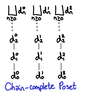
So, if we think back to any of the diagrams we drew previously, anywhere there was a “...’, in fact we could have placed an upper bound on the top of, courtesy of Haskell’s laziness. Here is one chain in the list type that has a least upper bound:
As we saw earlier, this is not always true for all partial orders, so we have a special name for posets that always have least upper bounds: chain-complete posets, or CPOs.
You may have also noticed that in every diagram, ⊥ was at the bottom. This too is not necessarily true of partial orders. We will call a CPO that has a bottom element a domain.
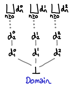
(The term domain is actually used quite loosely within the denotational semantics literature, many times having extra properties beyond the definition given here. I’m using this minimal definition from Marcelo Fiore’s denotational semantics lectures, and I believe that this is the Scott conception of a domain, although I haven’t verified this.)
So we’ve been in fact dealing with domains all this time, although we’ve been ignoring the least upper bounds. What we will find is that once we consider upper bounds we will find a stronger condition than monotonicity that entails computability.
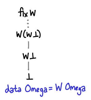
Consider the following Haskell data type, which represents the vertical natural numbers Omega.
Here is a monotonic function that is not computable.
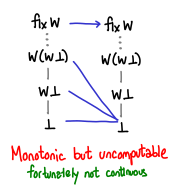
Why is it not computable? It requires us to treat arbitrarily large numbers and infinity different: there is a discontinuity between what happens on finite natural numbers and what happens at infinity. Computationally, there is no way for us to check in finite time that any given value we have is actually infinity: we can only continually keep peeling off Ws and hope we don’t reach bottom.
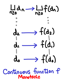
We can formalize this as follows: a function D -> D, where D is a domain, is continuous if it is monotonic and it preserves least upper bounds. This is not to say that the upper bounds all stay the same, but rather that if the upper bound of e_1 ≤ e_2 ≤ e_3 ... is lub(e), then the upper bound of f(e_1) ≤ f(e_2) ≤ f(e_3) ... is f(lub(e)). Symbolically:
 = \bigsqcup_{n \ge 0} f(d_n)")
Pictorially:
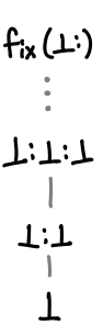
Now it’s time to look at fixpoints! We’ll jump straight to the punchline: Tarski’s fixpoint theorem states that the least fixed point of a continuous function is the least upper bound of the sequence ⊥ ≤ f(⊥) ≤ f(f(⊥)) ...
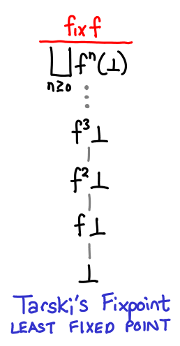
Because the function is continuous, it is compelled to preserve this least upper bound, automatically making it a fixed point. We can think of the sequence as giving us better and better approximations of the fixpoint. In fact, for finite domains, we can use this fact to mechanically calculate the precise fixpoint of a function.
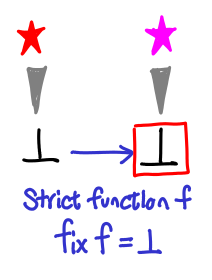
The first function we’ll look at doesn’t have a very interesting fixpoint.
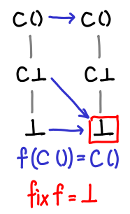
If we pass bottom to it, we get bottom.
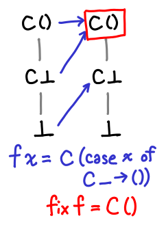
Here’s a slightly more interesting function.
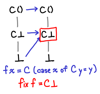
It’s not obvious from the definition (although it’s more obvious looking at the Hasse diagrams) what the fixpoint of this function is. However, by repeatedly iterating f on ⊥, we can see what happens to our values:
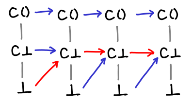
Eventually we hit the fixpoint! And even more importantly, we’ve hit the least fixpoint: this particular function has another fixpoint, since f (C ()) = C ().
Here’s one more set for completeness.
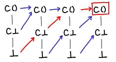
We can see from this diagrams a sort of vague sense why Tarski’s fixpoint theorem might work: we gradually move up and up the domain until we stop moving up, which is by definition the fixpoint, and since we start from the bottom, we end up with the least fixed point.
There are a few questions to answer. What if the function moved the value down? Then we might get stuck in an infinite loop.
We’re safe, however, because any such function would violate monotonicity: a loop on e₁ ≤ e₂ would result in f(e₁) ≥ f(e₂).
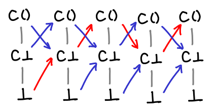
Our finite examples were also total orders: there was no branching of our diagrams. What if our function mapped a from one branch to another (a perfectly legal operation: think not)?
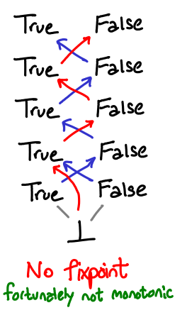
Fortunately, in order to get to such a cycle, we’d have to break monotonicity: a jump from one branch to another implies some degree of strictness. A special case of this is that the fixpoints of strict functions are bottom.
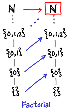
The tour de force example of fixpoints is the “Hello world” of recursive functions: factorial. Unlike our previous examples, the domain here is infinite, so fix needs to apply f “infinitely” many times to get the true factorial. Fortunately, any given call to calculuate the factorial n! will only need n applications. Recall that the fixpoint style definition of factorial is as follows:
factorial = fix (\f n -> if n == 0 then 1 else n * f (n - 1))
Here is how the domain of the factorial function grows with successive applications:
The reader is encouraged to verify this is the case. Next time, we’ll look at this example not on the flat domain of natural numbers, but the vertical domain of natural numbers, which will nicely tie to together a lot of the material we’ve covered so far.